Analysis of air flow over bicycle using Python
Objective:
Write a Python program to calculate drag force against a cyclist with respect to different factors involved.
The factors involved are Velocity,Drag coefficient,Frontal Area,Density of air.
Case-1: Program to plot Velocity vs Drag force.
Case-2: Program to plot Drag Co-efficient vs Drag force.
Drag Force:
The force on an object that resists its motion through a fluid is called ‘drag’. A drag force acts in opposition to the direction of motion and therefore has a negative effect on the velocity. For most large objects such as bicyclists, cars, and baseballs not moving too slowly, the magnitude of the drag force FD is found to be proportional to the square of the speed of the object. We can write this relationship mathematically as
`underset(D)Fpropv^2`
When other factors are taken into account, this relationship becomes
`underset(D)F= 1/2 rho A v^2 underset(D)C`
where
 is the drag force (N)
 is the mass density of the fluid `((kg)/m^3)`
v is the flow velocity relative to the object (m/s)
A is the reference area `(m^2)`
and  is the drag coefficent (unit-less)
Case-1: Program to plot Velocity vs Drag force.
While plotting the Velocity vs Drag force graph, A , ρ and Cd remains constant.
Backup Position of cyclist is considered.
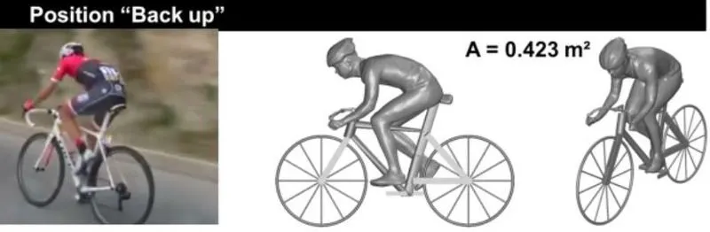
Density of Air `(rho) = 1.2 (kg)/m^3`
Frontal Area `(A)= 0.423 m^2`
Coefficient of drag = 0.70
Velocities (V) = 1 to 20 m/s with 1 interval
Python Code:
"""
Analysis of flow over bicycle for drag force calculation_Case-1 by Giridhar
"""
import math
import matplotlib.pyplot as plt
# inputs
# Drag coefficient
c_d = 0.7
# Frontal area(m^2)
A = 0.423
# Density(kg/m^3)
rho = 1.2
# Velocity(m/s)
velocities = [1,2,3,4,5,6,7,8,9,10,11,12,13,14,15,16,17,18,19,20]
drag_forces = []
for velocity in velocities:
	drag_forces.append(0.5*c_d*A*rho*pow(velocity,2))

print(drag_forces)
plt.plot(velocities,drag_forces)
plt.xlabel('velocity')
plt.ylabel('drag force')
plt.savefig('drag_force_flow_over_bicycle')
plt.show()
Output:

Velocity vs Drag Force Plot:
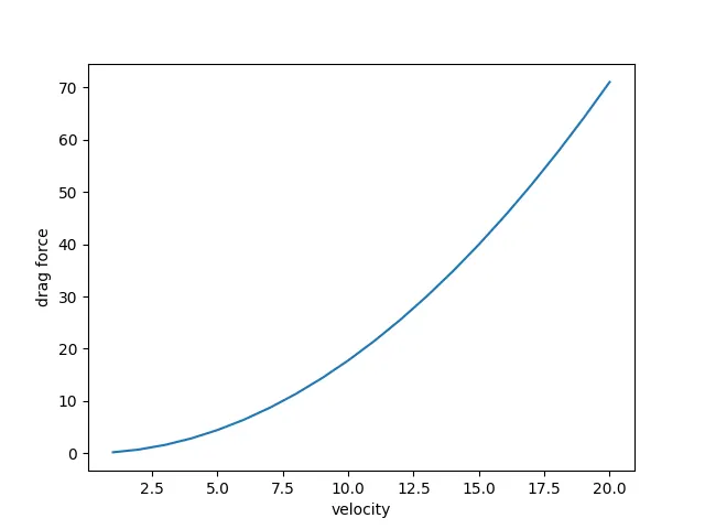
The curve is parabolic in shape. As the drag force is directly proportional to square of velocity, the curve is parabolic rather than linear.
The greater the velocity of a body through a fluid, the greater the drag force and drag force becomes four times as velocity doubles and can be observed from graph and output values. At the same time it justifies the mathematical relationship `underset(D)Fpropv^2`
Case-2: Program to plot Drag Co-efficient vs Drag force.
While plotting graph between the coefficient of drag vs drag force, A, ρ and V remains constant.
Density of Air `(rho) = 1.2 (kg)/m^3`
Velocity (v) = 12 m/s
Frontal Area `(A)= 0.423 m^2`
Coefficient of drag = [0.588, 0.6, 0.611, 0.637, 0.64, 0.645, 0.65, 0.67, 0.68, 0.70]
| S.No. | Position | Picture | |
| 1 | Top Tube 3 | 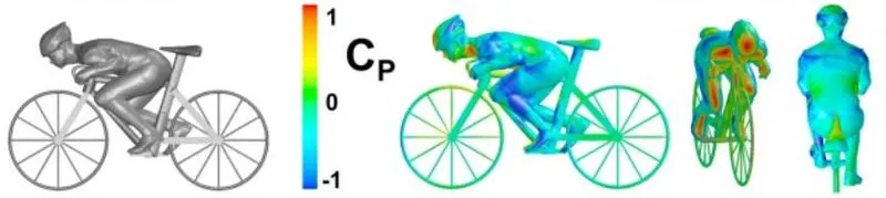 |
0.588 |
| 2. | Top Tube 4 | 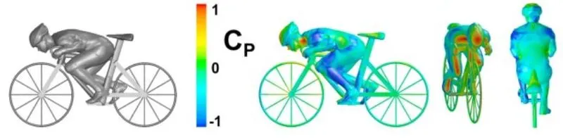 |
0.60 |
| 3. | Top Tube 2 | 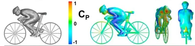 |
0.611 |
| 4 | Back Horizontal | 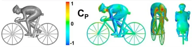 |
0.637 |
| 5 | Back Down 2 | 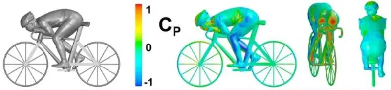 |
0.64 |
| 6 | Top Tube 1 | 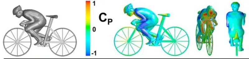 |
0.645 |
| 7 | Back Down 1 | 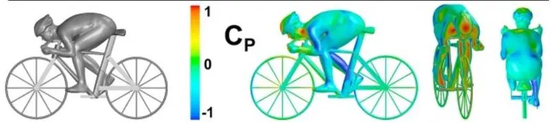 |
0.65 |
| 8 | Elbows | 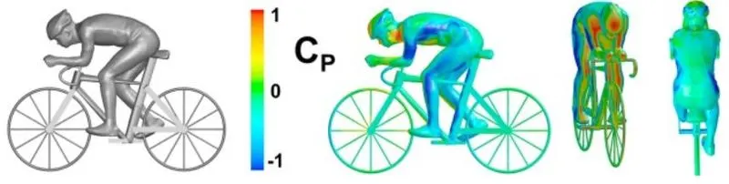 |
0.67 |
| 9 | Froome | 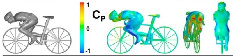 |
0.68 |
| 10 | Backup | 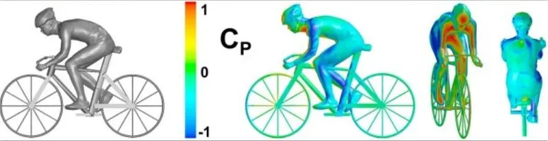 |
0.7 |
Even though the frontal area and coefficient of drag changes with change in shape. Frontal area is considered constant with `A= 0.423 m^2`and drag coeffcient is changed as per shape.
Python Code:
"""
Analysis of flow over bicycle for drag force calculation_Case-2 by Giridhar
"""
import math
import matplotlib.pyplot as plt
# inputs
# Drag coefficient
c_d10 = [0.588, 0.6, 0.611, 0.637, 0.64, 0.645, 0.65, 0.67, 0.68, 0.70]
# Frontal area(m^2)
A = 0.423
# Density(kg/m^3)
rho = 1.2
# Velocity(m/s)
velocity = 12
drag_forces = []
for c_d in c_d10:
	drag_forces.append(0.5*c_d*A*rho*pow(velocity,2))

print(drag_forces)
plt.plot(c_d10,drag_forces)
plt.xlabel('Drag Coefficient')
plt.ylabel('drag force')
plt.savefig('drag_force_flow_over_bicycle_Case2')
plt.show()
Output:

Drag Coeffcient vs Drag Force Plot:
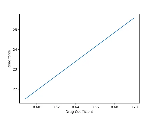
The value of drag force increases with an increase in value of coefficient of drag linearly.
Code Explanation:
- Math module is imported as the code contains mathematical calculations.
- matplotlib.pyplot as plt is imported as we need plots from the calculations performed.
- Inputs required are given.
- Velocity in Case-1 and Drag coefficient in Case-2 is given in the form of arrays to calculate drag forces for different values of inputs respectively.
- Drag forces is defined using a empty array for output.
- A for loop is created to create various plots for incremental changes for respective values.
- Append is used to calculate drag forces for the given number of inputs.
- print command is used to get drag forces.
- plt.plot is used to plot drag forces vs velocity or drag coefficient.
- x label and y label is defined using plt._label.
- The plot is saved using plt.savefigure and the same is shown using plt.show command.
References:
All Pics Credit: https://www.sciencedirect.com/science/article/pii/S0167610518305762
c. https://www.sciencedirect.com/science/article/pii/S0167610518305762