AIR STANDARD CYCLE (OTTO CYCLE) USINGH PYTHON

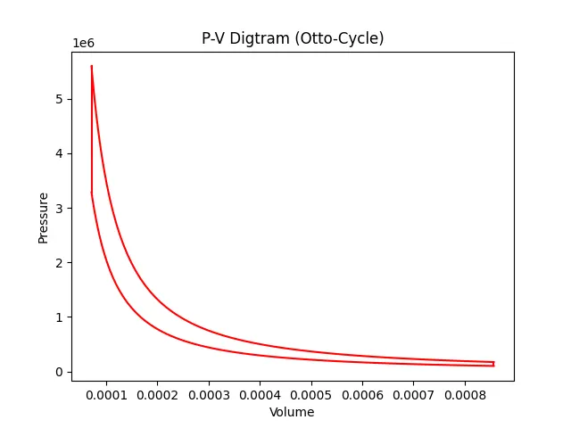
The object of the Project: - In this project, we calculate the Pressure and Volume of various points, efficiency, and plot the P-V Diagram (Otto Cycle) for a 4-stroke petrol engine using “Python” programming.

Otto Cycle and Process: - The Otto cycle is the ideal cycle for spark-ignition engines, in honor of Nikolaus Otto, who invented it in 1867. In ideal Otto cycles, the air-standard assumption is used. The ideal Otto cycle consists of four internal reversible processes:

• 1-2 Isentropic compression process
• 2-3 Constant volume heat addition process
• 3-4 Isentropic expansion process
• 4-1 Constant volume heat rejection process

Formula of

Efficiency of an ideal Otto cycle: - an ideal thermodynamic combustion cycle, as follows: a compression at constant entropy; a constant-volume heat transfer to the system; an expansion at constant entropy; and a constant-volume heat transfer from the system. The thermal efficiency of the ideal Otto cycle increases with an increasing compression ratio.

`eta = 1 - 1/ (C_r^(gamma-1)`

Main Program: -

# Otto Cycle
import math
import matplotlib.pyplot as plt

#Engine Kinmetics Function for Volume Changing Various point
def Engine_kinematics(bore,stroke,con_rod,Cr,start_crank,end_crank):
    a = stroke/2
    R = con_rod/a
    sc = math.radians(start_crank)
    ec = math.radians(end_crank)
    value = 100
    dtheta =  (ec-sc)/(value-1)
    V = []
    for i in range(0,value):
        theta = sc + i*dtheta
        term1 = 0.5*(Cr-1)
        term2 = R+1-math.cos(theta)
        term3 = math.sqrt(pow(R,2)-pow(math.sin(theta),2))
        V.append(Vc*(1 + term1*(term2-term3)))
    return V

#Inputs
P1  = 101325    #Pressure at poinnt  1 (N/m^2)
t1 = 500        #Temperature at point 1 (K)
gamma = 1.4     #Specific heat ratio(gamma)
t3 = 2300       #Temperature at point 3 (K)

#Gemotry Parameter
bore = 0.1
stroke = 0.1
con_rod = 0.18  #Connecting Rod length (m)
Cr = 12         #Compression ratio

#Volume Computation
Vs = (math.pi/4)*pow(bore,2)*stroke     #Swept volume 
Vc = Vs/(Cr - 1)                        #Clearance volume
V1 = Vs + Vc                            #Total cylinder volume

#State point 2
V2 = Vc                                                          
#P2V2^gamma = P1V1^gamma
P2 = P1*pow((V1/V2), gamma)             #Pressure at point-2(N/m^2)
#P2V2/t2 = P1V1/t1
t2 = P2*V2*t1/(P1*V1)                   #Temperature at point 2 (K)
#Point(1-2) Adiabatic Compression Process
V_compression = Engine_kinematics(bore,stroke,con_rod,Cr,180,0)
constant = P1*pow(V1,gamma)
P_compression = []                      
for v in V_compression:
    P_compression.append(constant/pow(v,(gamma)))

#State point 3
V3 = V2                                 #Point(2-3)constant Volume Process
#P3V3/t3 = P2V2/t2
P3 = P2*V2*t3/(V3*t2)                   #Pressure at point-3(N/m^2)
#Point(3-4)Adiabatic Expansion Process
V_expansion = Engine_kinematics(bore,stroke,con_rod,Cr,180,0)
constant = P3*pow(V3,gamma)
P_expansion = []
for v in V_expansion:
    P_expansion.append(constant/pow(v,(gamma)))

#State Point 4                           
V4 = V1                                 #Point(4-1)constant Volume Process
#P4V4^gamma = P3V3^gamma
P4 = P3*pow((V3/V4),gamma)              #Pressure at point-4(N/m^2)
#P4V4/t4 = P3V/t3
t4 = P4*V4*t3/(P3*V3)                   #Temperature at point 4 (K)
eta = (1-1/Cr**(gamma-1))*100           #Air standard efficiency
print('Efficiency = %.2f'%(eta),"%")
plt.plot([V2,V3],[P2,P3],color="red")
plt.plot([V4,V1],[P4,P1],color="red")
plt.plot(V_compression,P_compression,color="red")
plt.plot(V_expansion,P_expansion,color="red")
plt.xlabel('Volume')
plt.ylabel('Pressure')
plt.title('P-V Digtram (Otto-Cycle)')
plt.savefig('Otto_Cycle.png')              #To save plot figure
plt.show()

Problem Statement:-

1. I didn’t face any problem.

Solution: -

None

Result: -

Efficiency = 62.99 %