Ahmed Body Challenge
AIM : To simulate the flow over an Ahmed body and to calulcate the values of drag and lift co-efficients generated and to carry out the grid dependency test.
SIMULATION-SETUP :
- Case setup : ANSYS (FLUENT)
- Simulation editor : ANSYS FLUENT
- Post-processor : CFD POST
THEORY :
Air has a tendency to curl downwards around the ends of a car, travelling upwards from the high-pressure region under the car to the low-pressure region on top, at the rear end of the automobile and subsequently collides with moving low-pressure air. The kinetic energy of these turbulent air spirals acts in a direction that is negative relative to the direction of travel intended. Thus, the car engine must compensate for the losses created by this drag. Vortices are released during flow separation and trail downstream to form structured or unstructured wake patterns. A wake is the region of re-circulating flow immediately behind a moving or stationary solid body, caused by the flow of surrounding fluid around the body. The local disturbances in the flow pattern behind the vehicle causes a momentum loss thus causing form drag which extends far behind the bodyworks of a vehicle.
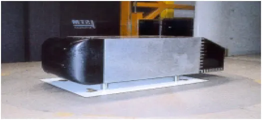
What Is an Ahmed Body?
Ahmed Body is an approximate shape of automotive vehicles (specifically a generic car model) used to capture the essential flow features like lift, drag, wake regions and all, around the body when it is moving through a fluid (air).
The simple geometrical shape has a length of 1.044 meters, height of 0.288 meters, and a width of 0.389 meters. It also has 0.3-meter cylindrical legs attached to the bottom of the body and the rear surface has a slant that falls off at 35 degrees (slant angle).
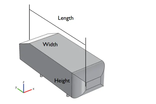
Why Study the Drag Coefficient in Cars?
The drag-coefficient quantifies the resistance of an object in a fluid environment. It is not an absolute constant for a body’s shape because it varies with the speed and direction of flow, object shape and size, and the density and viscosity of the fluid. The lower the drag coefficient of an object, the less aerodynamic or hydrodynamic drag occurs. In terms of a car, the lower the drag coefficient, the more efficient the car is. As well as affecting the top speed of a vehicle, the drag coefficient also affects the handling. Cars with a low drag coefficient are sought after, but decreasing the drag drastically can reduce the down force and lead to loss in road traction and a higher chance of car accidents.
CREATING A VIRTUAL W IND TUNNEL :
A wind tunnel is an aerodynamic facility to visualize the flow over an external surface. Designing the wind tunnel for any model is a crucial point in any CFD analysis and if the design parameters go wrong, we’ll end up in a wrong simulated answers. Hence setting up a good wind tunnel is a crucial point in any CFD analysis.
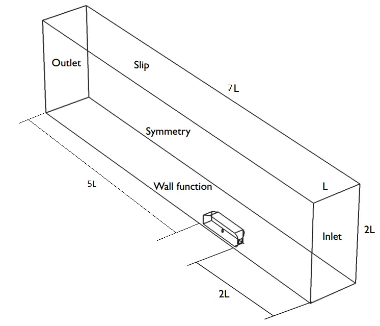
JUSTIFICATION FOR ABOVE MENTIONED PARAMETERS :
A question arises, why should some-one give the above mentioned dimensions only?? Well the answer is quite simply, initially the flow at the inlet will have a uniform velocity profile, once the flow starts or starts accelerating there will be a development of boundary layer due to the wall in the wind-tunnel.
Well, why does the boundary layer develops??
It is due to the effect called “ coanda effect ”. It says that the fluid jet has a tendency to remain attached to the surface (convex) of the body. So when there is a small region of fluid flow, there will be a development of viscosity. Viscosity is the resistance offered by the fluid for it’s flow, the reason for development of viscosity and viscous forces is ‘shear stresses’.
Hence boundary layer is a region of small fluid flow where viscous forces are dominant, hence to capture theses effects the length should be logically acceptable and that’s the reason for inflow length.
When we come to the outflow side , as discussed above the flow has a tendency to curl according to the geometry of the body, so when the flow encounter any curvatures or complex shaped, the behavior of flow is entirely different. When the flow separates from the body , it leads to formation of vortices. Vortices are then released downstream of the body leading to the formation of structured or unstructured ‘wake patterns’.
Wake is a region of re-circulation where the flow re-circulates and it is the zone of low-pressure. All this happenes because of the drop in the static pressure.
In the region of re-circulation ie,, wake, we don’t know what is the velocity of the flow there and hence to captures all this things, we need to position the body from the outlet at sufficient length, so that the flow can straighten out and come back to the free-stream conditions, where we can then get to know the velocity of the flow in the wake region accurately.
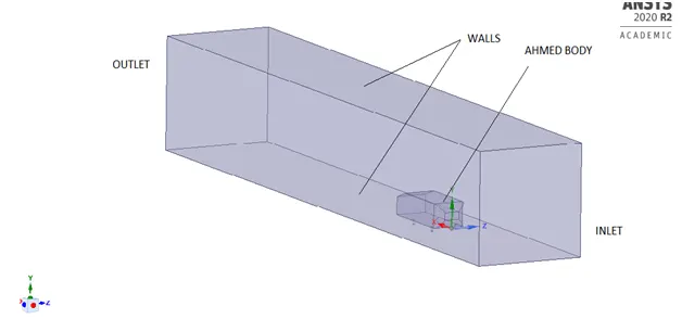
Above figures shows the modeling of virtual wind tunnel in converge. The Ahmed Body has a length (L) of 1.044m and a height of 0.288m and width of 0.389m, with frontal area being
BOUNDARY FLAGGING AND BOUNDARY CONDITIONS :
The geometry was flagged into different boundaries and suitable boundary conditions were assigned to it.
- INLET – Inlet is an inflow type boundary condition assigned, since we know the velocity, the velocity condition will be a Dirchlet boundary condition (DI) , with velocity being 40 m/s and pressure being a Nueman boundary condition (NE)
- OUTLET – Outlet is an outflow type boundary condition assigned, with pressure being specified as Dirchlet boundary condition (DI) of 1 atm.
- FRONT_BACK_TOP_BOTTOM_SURFACES – All these surfaces were assigned to a symmetry boundary conditions, since we want the flow properties to be same on both the sides and also for a 2D simulation front and back are just walls.
- AHMED BODY : Since the main aim of doing the simulation is over this body, ‘law of wall boundary’ condition was selected as formation of boundary layer was required in this region.
WRITING TIME INTERVALS AND TURBULENCE MODELLING :
The simulation ran was a steady state simulation starting from zero iteration till the convergence of the solution. (around 1000 iterations)
Turbulence modelling :
The turbulence model used here is ‘ k−ωSST ’
- This turbulence model is the combination of RNGk−ε and Standard k−ω And hence it near the wall ‘k−ωSST ’ works as a Standard k−ω model and away from the wall it works RNGk−ε model.
- Hence it gives an accurate prediction near the wall and away from the wall, as we are interested in capturing boundary layer growth.
Also k−ωSST model is well known for it’s automatic wall-treatment, which captures boundary layer accurately.
MESHING :
The simulation was done for three different cases ie,,, for a base-line mesh and the remaining two for a finer mesh.
CASE 1 : Base-line meshing (element size -400mm )
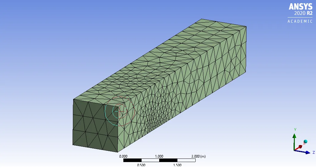
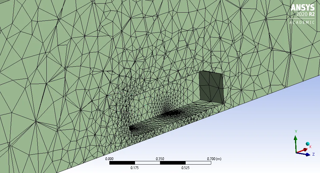
83781 triangular elements were created in this case.
SIMULATION RESULTS :
1) DRAG FORCE AND COEFFICEINT :
Drag force :
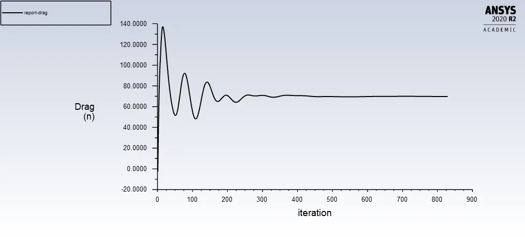
The value of drag force was found to be converged around 69.763 N for an inlet velocity of 25 m/s and pressure being 1atm.
Drag co-efficient :
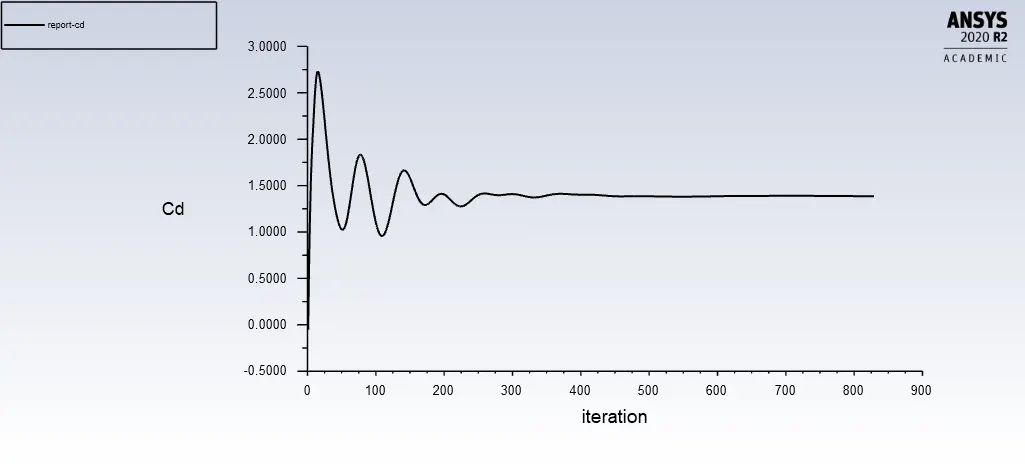
The value of drag coefficient was found to be 1.34 for an inlet velocity of 25 m/s.
2) LIFT FORCE AND COEFFICIENT :
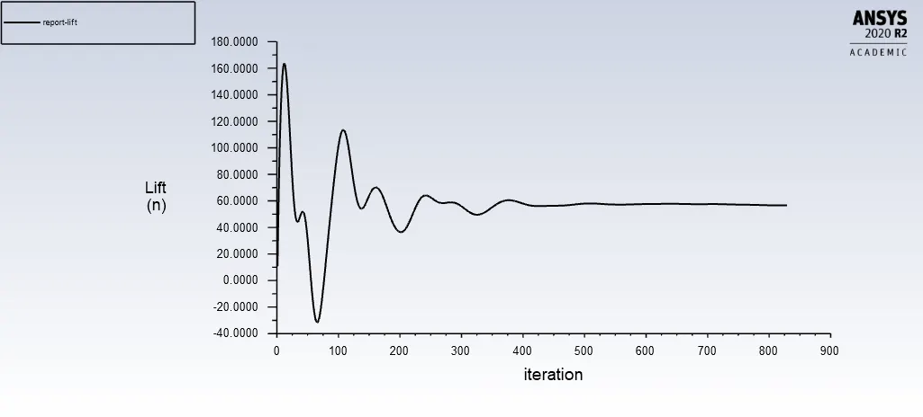
The value of lift force converged for 56.67N a for an inlet velocity of 25 m/s.
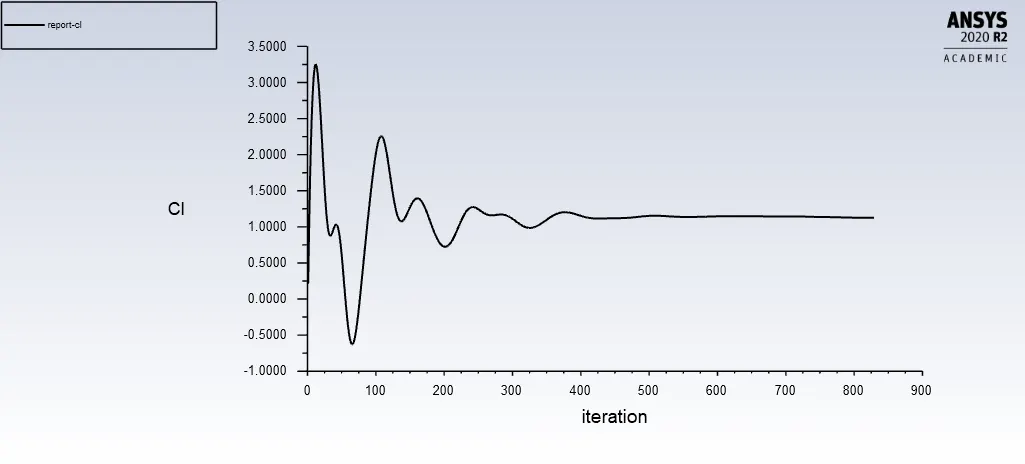
The value of lift coefficient was found to be 1.25.
RESIDUALS :
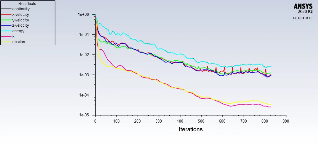
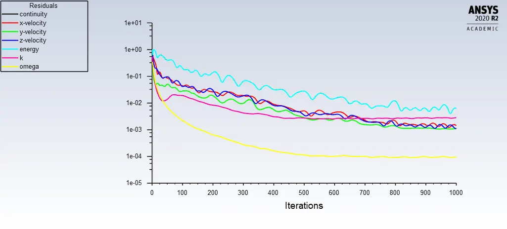
Residuals are the set of governing equations that governs the fluid flow simulation. Above figure shows the plot of residuals and their variations in the
simulation.
Now let us refine the above case setup for better and accurate results and let us the run the simulation for the refined mesh.
The refined mesh consists of :
1) Inflation layers : layers around the ahmed body with total thickness for better aerodynamic accuracies.
2) Multi-zone : Modifying the elements in the mesh from triangular to hexahedral meshing elements.
3) Sizing : Allows us to have a control over the elements to be modified in the simulation.
CASE 2 : Finer meshing (element size -80mm )
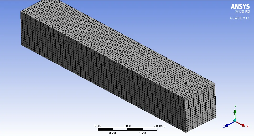
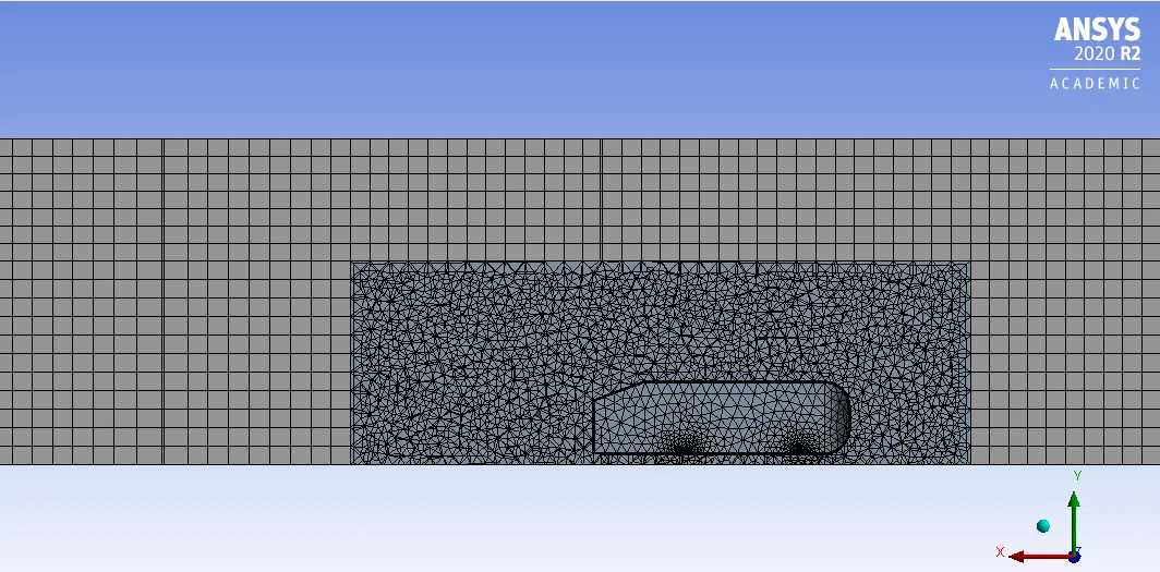
320189 hexahedral elements were created in this case. Hexahedral elements are better suited for refinement as they have a symmetric profile and gives the accurate results during simulation.
SIMULATION RESULTS :
1) DRAG FORCE AND COEFFICEINT :
Drag force :
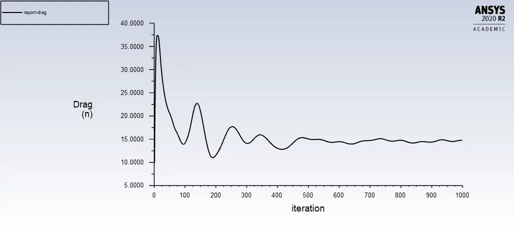
The value of drag force was found to be converged around 14.712 N for an inlet velocity of 25 m/s and pressure being 1atm.
Drag co-efficient :
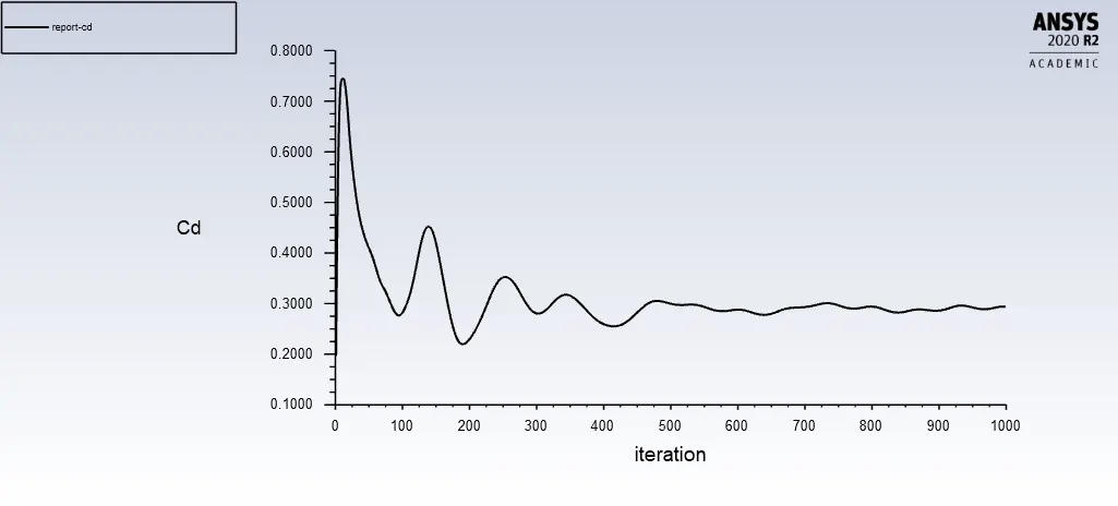
The value of drag coefficient was found to be 0.2936 for an inlet velocity of 25 m/s.
2) LIFT FORCE AND COEFFICIENT :
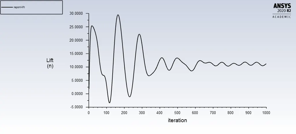
The value of lift force converged for 11.627N a for an inlet velocity of 25 m/s.
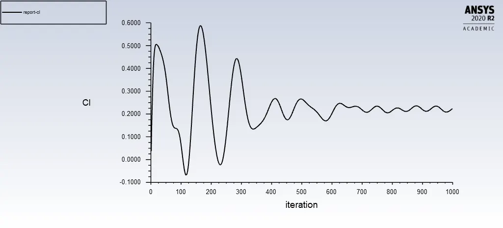
The value of lift coefficient was found to be 0.2244.
RESIDUALS :
CFD POST-PROCESSING RESULTS :
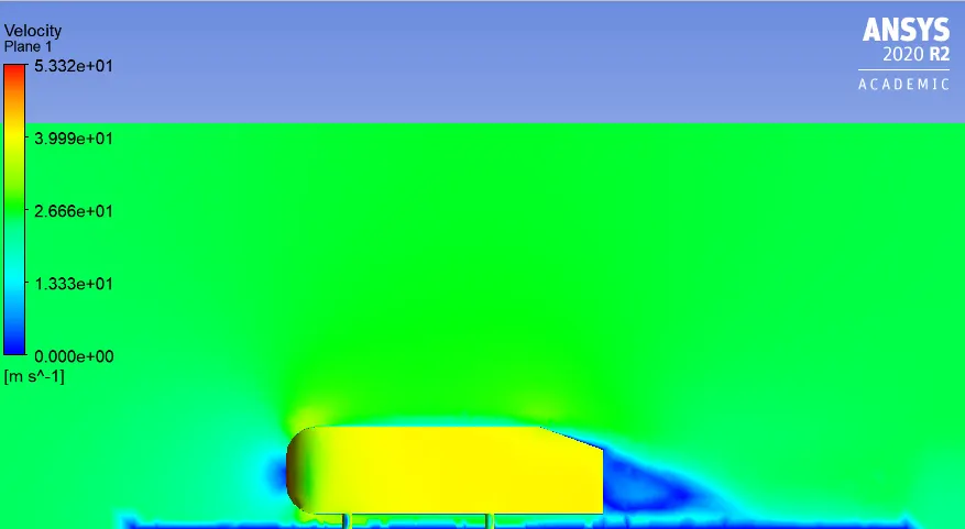
VELOCITY CONTOUR :
VECTOR AND STREAM LINE PLOT :
To depict the flow behaviour and to visualize the wake region it is neccessary for us to know how the flow behaves. Hence the vector and streamline (imaginary lines)
are plotted to depict it's behaviour.
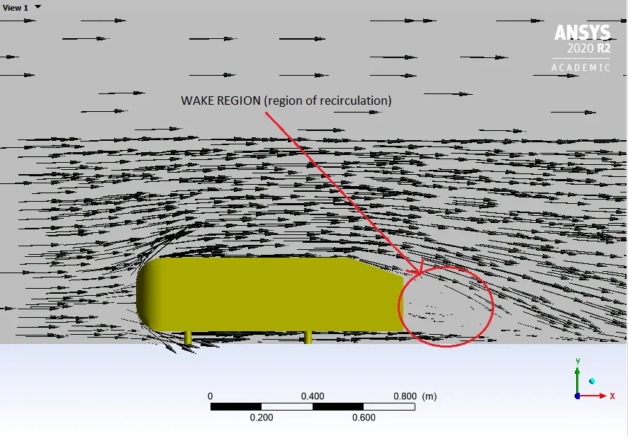
Above figure shows the vector plot. Wake is a region of low pressure where the recirculation of the flow takes places, hence it is known as recirculation region. The reason it
is also called as low pressure region is due to drop in static pressure (ie,, the flow pressure)
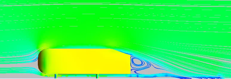
Above stream line fugure clearly shows the wake region (recirculation zone).
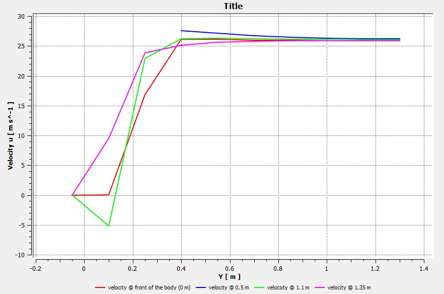
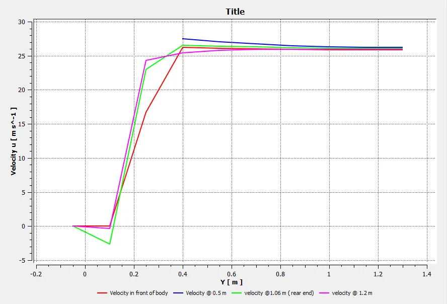
PLOT OF VARIATION OF VELOCITY w.r.t DISTANCE IN THE Y-AXIS OF THE BODY
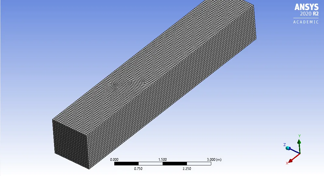
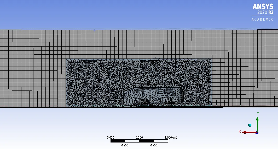
CASE 3 : Finer meshing (element size -70mm )
INFLATION LAYERS :
Around 6 infltion layers with growth rate of 1.2 in each case was added.
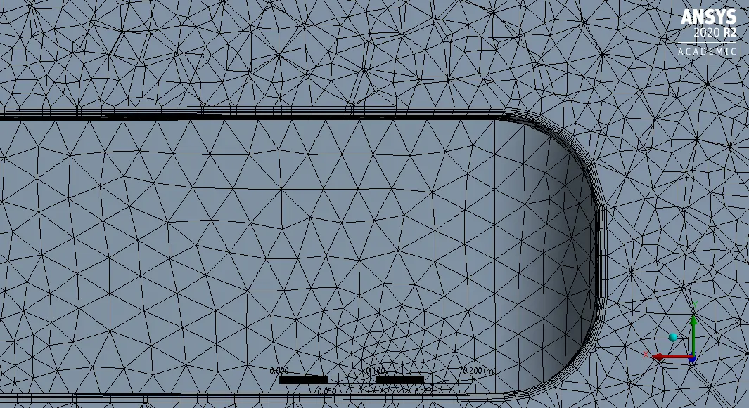
496229 hexahedral elements were created in this case.
SIMULATION RESULTS :
1) DRAG FORCE AND COEFFICEINT :
Drag force :
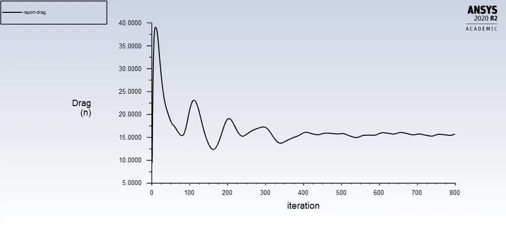
The value of drag force was found to be converged around 5.763 N for an inlet velocity of 25 m/s and pressure being 1atm.
Drag co-efficient :
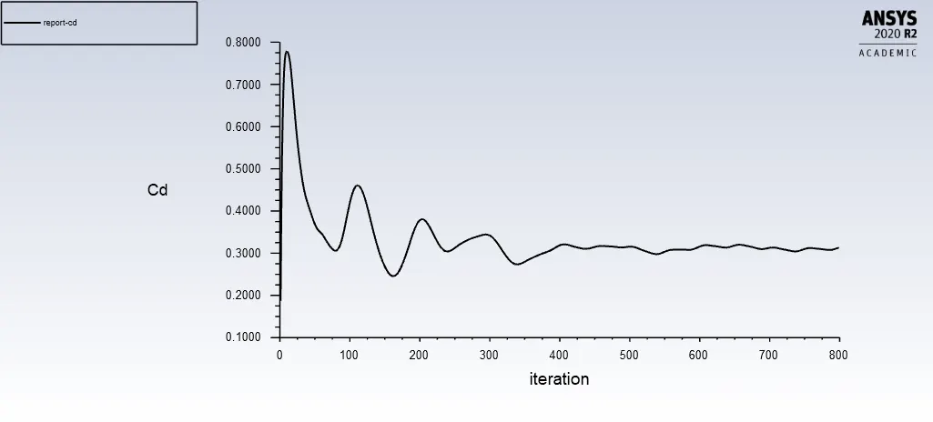
The value of drag coefficient was found to be 0.323 for an inlet velocity of 25 m/s.
2) LIFT FORCE AND COEFFICIENT :
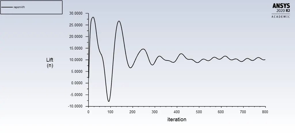
The value of lift force converged for 5.0123N for an inlet velocity of 25 m/s.
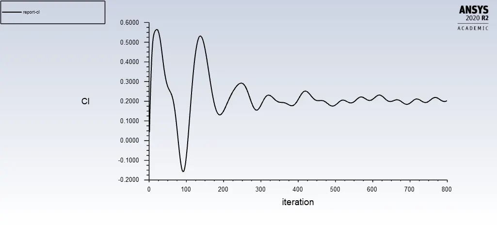
The value of lift coefficient was found to be 0.2178.
RESIDUALS :
CFD POST-PROCESSING RESULTS :
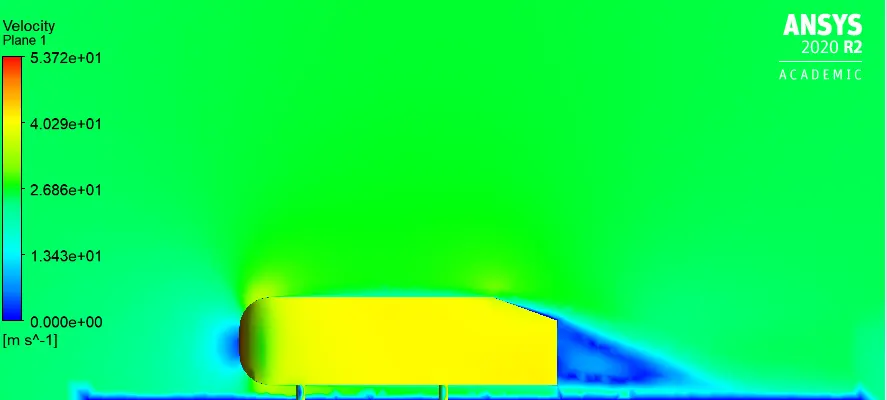
VELOCITY CONTOUR :
VECTOR AND STREAM LINE PLOT :
To depict the flow behaviour and to visualize the wake region it is neccessary for us to know how the flow behaves. Hence the vector and streamline (imaginary lines)
are plotted to depict it's behaviour.
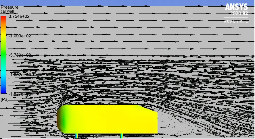
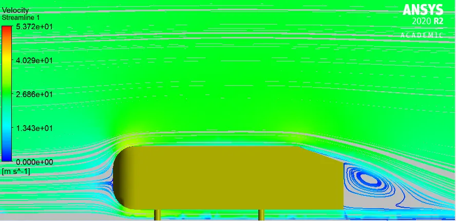
Above stream line figure clearly depicts the wake region.
PLOT OF VARIATION OF VELOCITY w.r.t DISTANCE IN THE Y-AXIS OF THE BODY
RESULTS AND INFERENCE :
The total drag coefficient of the Ahmed body is the key measurement for this simulation. It is made up of measurements for the pressure coefficients in the front, slant, and base of the body as well as the body’s skin friction. In the results of our simulation, the total drag is very well predicted but the individual measurements deviate from the experimental results in varying amounts. For a slant angle of 35-degree the value of drag and lift coefficients are found to be 0.3234 and 0.2178
Hence, from the simulation
Cd = 0.3234
Cl = 0.2178
When the body is moving at 25 m/s (although the science of air moving around stationary body or body moving around the stationary air is same) it encounters a resistive foroce of 5.765 N ie,, the drag force.