Ahmed Body Challenge

• OBJECTIVE : To examine flow around ahmed body car model and investigate wake region behind car body for given specific velocity of car.

• Ahmed body and its importance :

• Ahmed body simplified generic model of car which was devloped by Ahmed .
• air flow around ahmed body captures the physics of flow and its features in autompbile industry.
• The simple geometrical shape has a length of 1.044 meters, height of 0.288 meters, and a width of 0.389 meters. It also has 0.5-meter cylindrical legs attached to the bottom of the body and the rear surface has a slant that falls off at 40 degrees.
• The Ahmed body is a benchmark model widely used in the automotive industry for validating simulation tools. The Ahmed body shape is simple enough to model, while maintaining car-like geometry features.
• when the car hits on road with high velocity then its nessesary to examine its lift and drag force and this its co-efficients too its allows to better aerodynamis performance without produces loss for car having boxy type geometry like hummer which have high drag co-efficient in terms of 0.5 and for car having stramline body shaped like mercedez having low drag co-efficient like 0.3 more the drag more the fuel required to burn in order to attain high effeciency.
• In terms of a car, the lower the drag coefficient, the more efficient the car is. As well as affecting the top speed of a vehicle, the drag coefficient also affects the handling. Cars with a low drag coefficient are sought after, but decreasing the drag drastically can reduce the downforce and lead to loss in road traction and a higher chance of car accidents.

• significance on the point of Flow sepration :

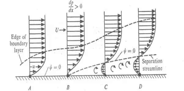
• when fluid passes through body because of higher momentum in starting its find favourable pressure difference (dp/dx < 0) which causes fluid to flow in upstream but while flowing its continue loosing its momentum transfer due to viscosity of fluid and induced shear stress when momentum transfer is not capable to overcome friction force due to shear stress at that point velocity and pressure gradient can be seen as zero ( dp/dx=0 & dv/dx=0 ) point at which flow septares and as flow further move in upward direction because of positive pressure gradient (dp/dx > 0 ) due to that adverse pressure difference fluid start to flow back and produces vortex.

• concept of wall y+ value :

• The y+ value is a non-dimensional distance (based on local cell fluid velocity) from the wall to the first mesh node, as you can see in the image below. To use a wall function approach for a particular turbulence model with confidence, we need to ensure that our y+ values are within a certain range.
• 
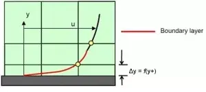
• Boundary layer is fluid region near the wall where viscous force are important , layer very close to wall where is fluid is pure viscous in nature and capture the flow very well is called as viscous sublayer
• as the boundary layer grows due to loss in momentum in order to overcome viscous effect where turbulent cames in picture and we can see mix of both layer called as buffer layer
• as boundary devloped more flow will be in turbulent nature fully called as log law layer or outer region

• its nesessary to select accurate and correct turbulent model
• for y+ value 0 to 5 where viscous sublayer llies a layer where capturing wall effect is more important in order to get netter accuracy K-w SST model is use.
• for y+ value > 100 where flow nature is turbulent k-eplison mmodel works better.
• one should avoid y+ value between 0 to 30 as buffer layer is present there.

• PROCEDURE :

After opening ansys workbench click on ansys fluent in toolbox and drag it into project schematic

1). Pre-procesing

2). Meshing.

3). Solving .

4). Post- processing.

1). Pre-procesing

• click on geometry in which change the settings of unit to meter .
• import geometry of ahmed body since we are simulating aerodynamics simulation its neccesary to have region in which we can investigate flow thus adding enclosure as shown below .

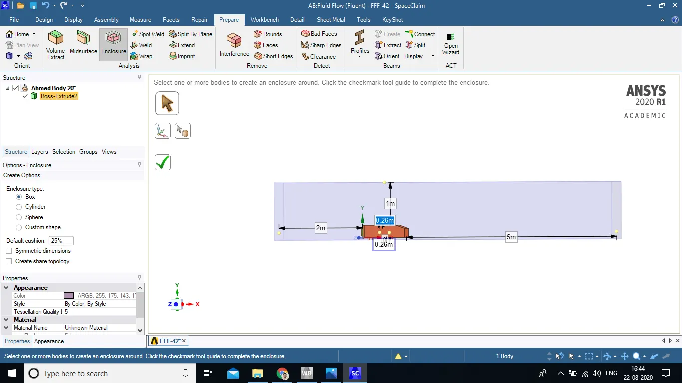
• by unchecking boss-extrude that means ahmed body will be subtracted from given inclosure area which can be seen by using cut plane (section ) with selecting appropriate plane

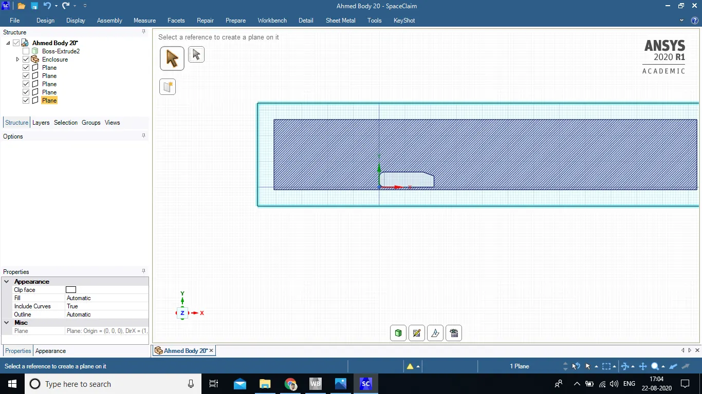
• while generating base line mesh setup its noticed theres mesh inside ahmed body which not feasible for our simulation .

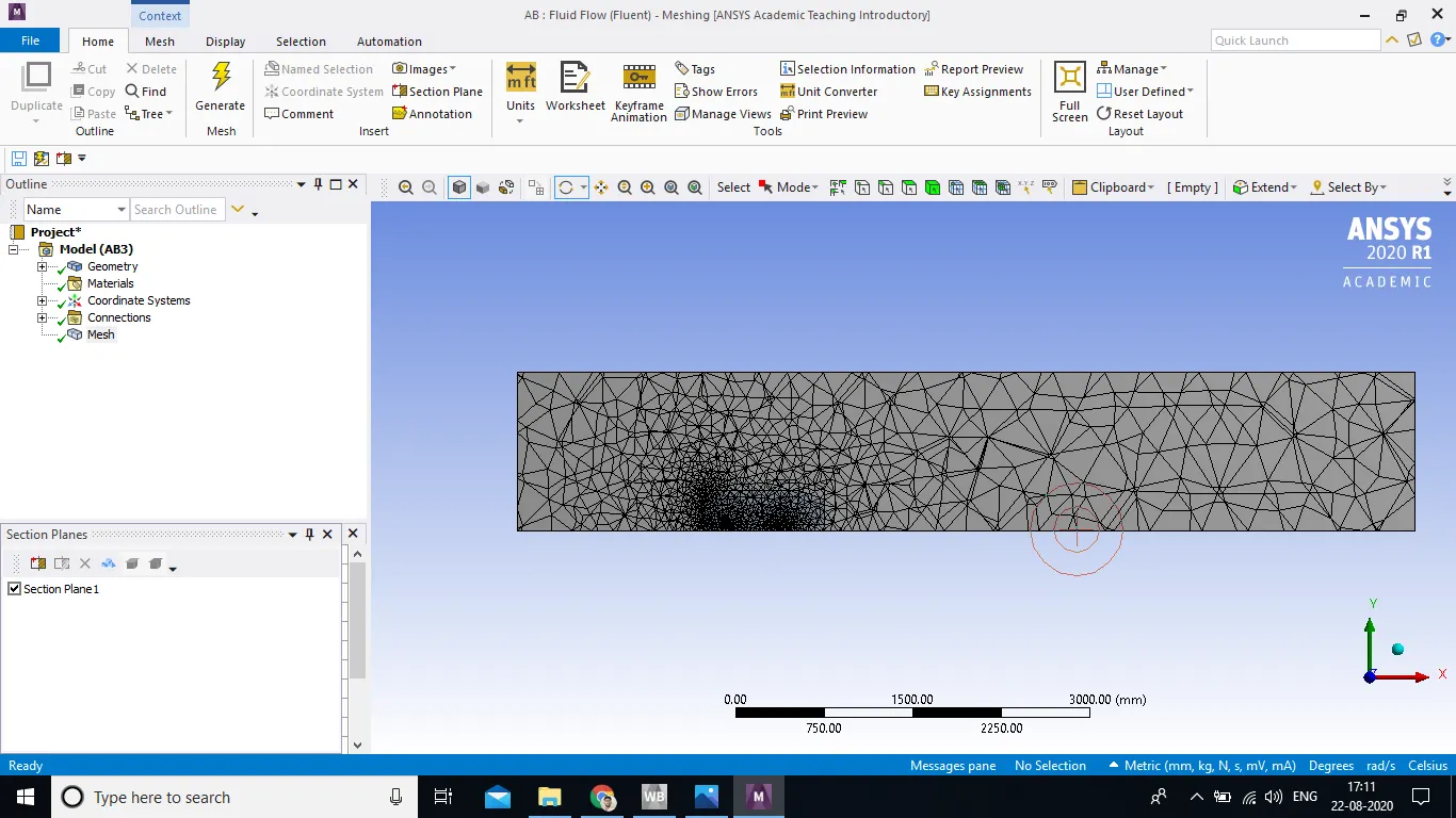
• Thus ahmed body need to supress for physics in order to remove the meshes from inside body.

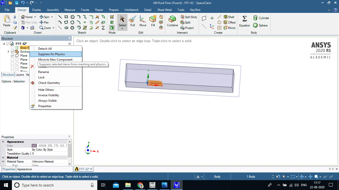
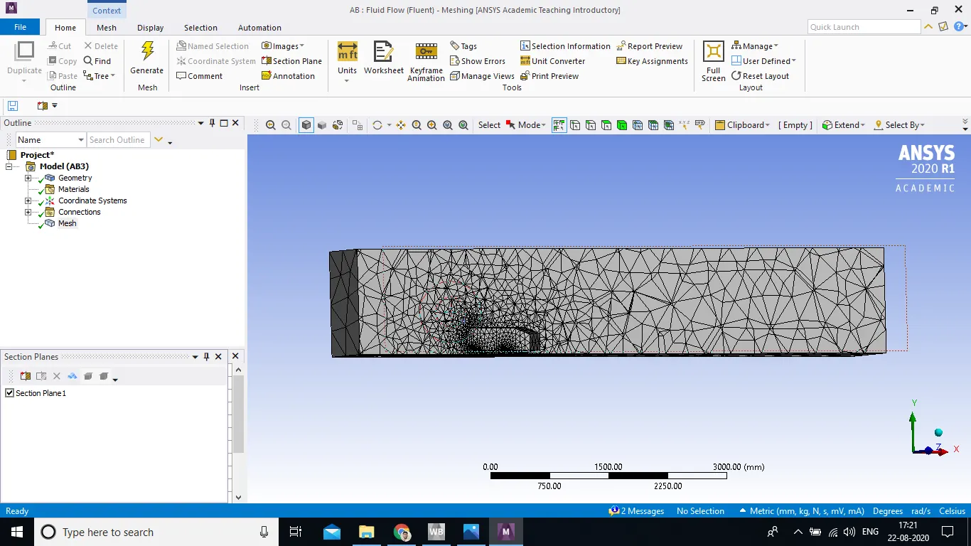
• it can be seen from below figure we have got geometry where mesh is not inside the ahmed body

• to capture physics better we are going add inner enclosure while adding enclosure tropology must be share inorder to prevent mesh from inner enclosure to outer inclosure as shown in below

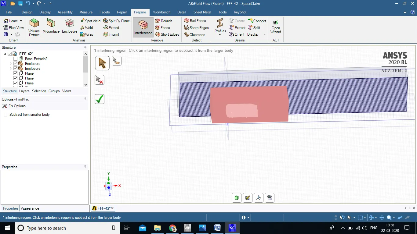
• with use of inteference command hatch line which are mating with respective can be seen and then share tropology.

2). Meshing.

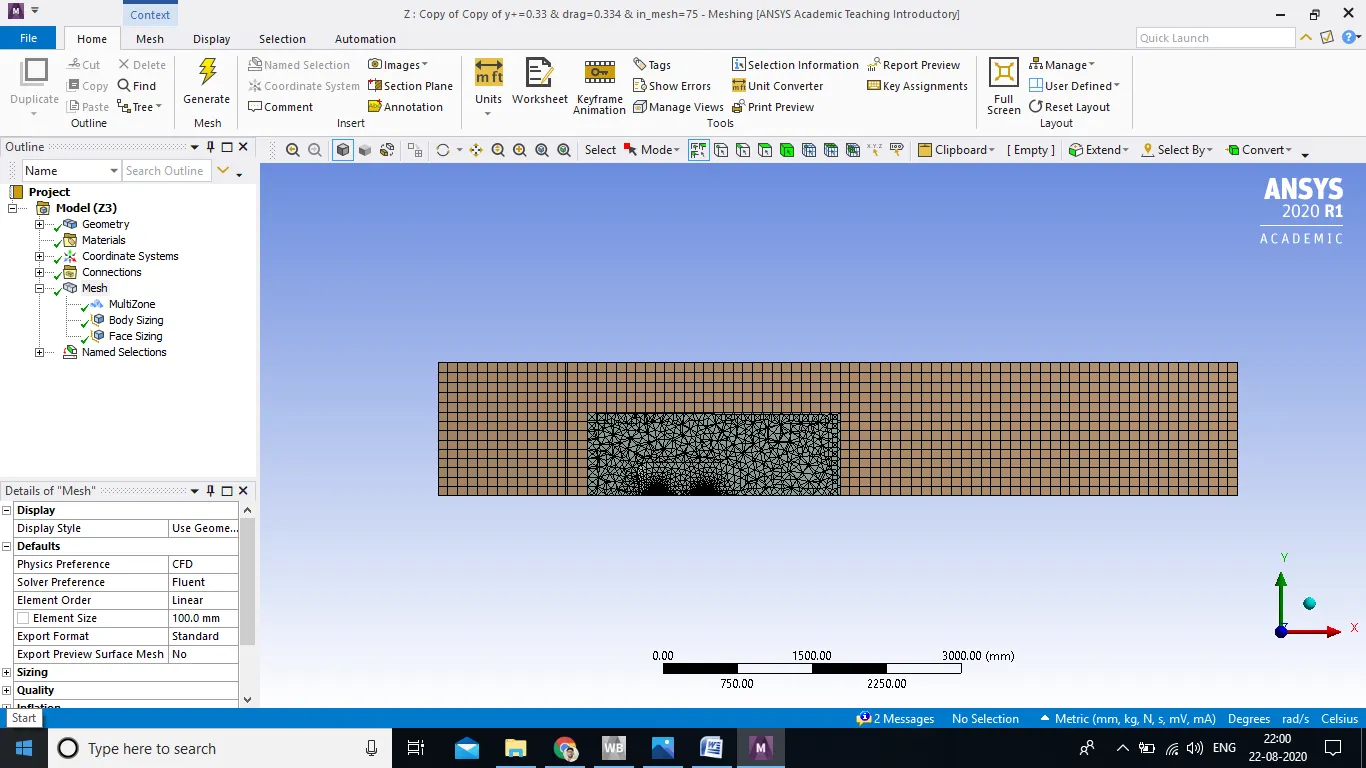
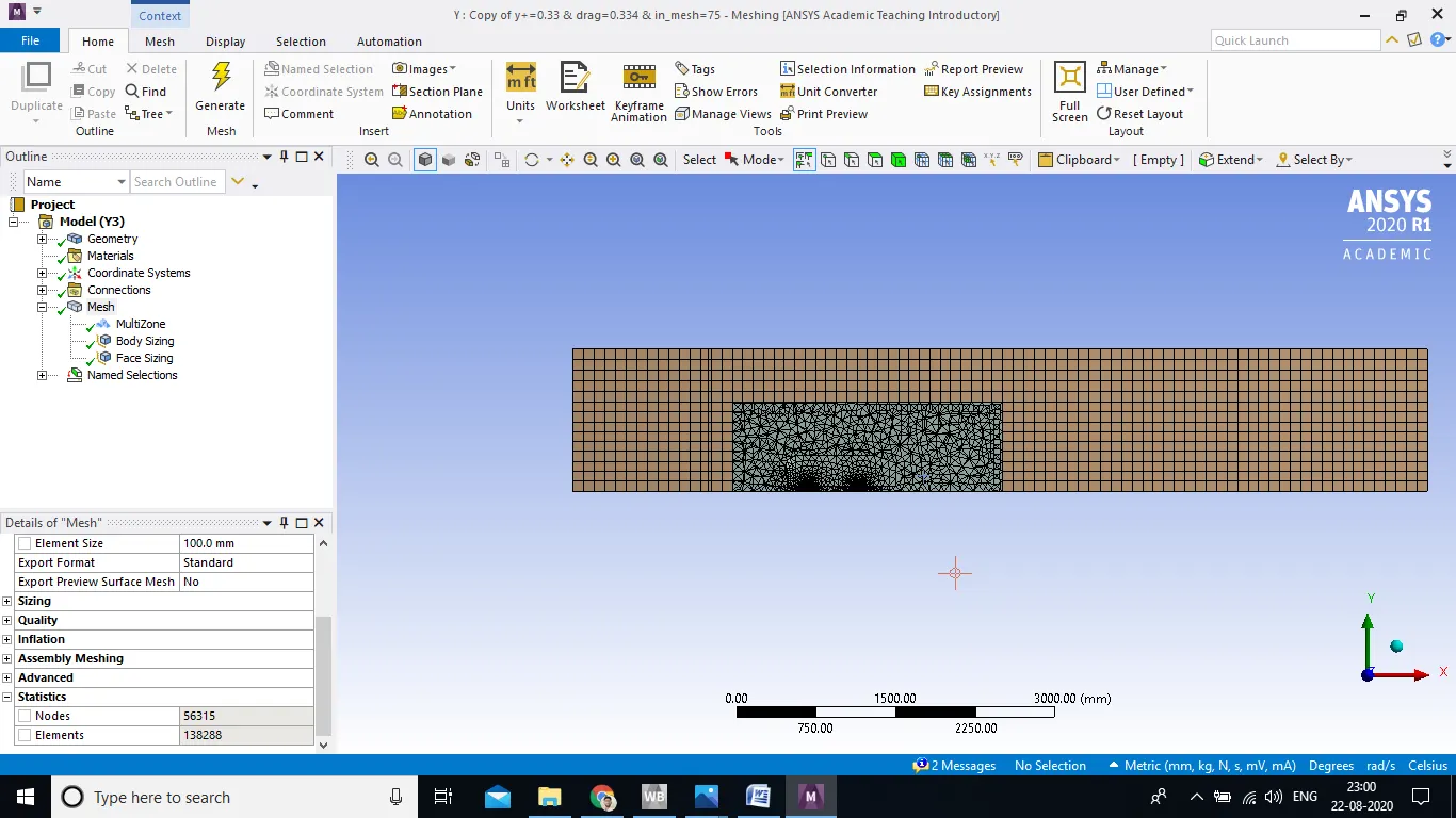
• geometry where shape is like boxy then hexa mesh should use . select multizone and create mesh which will create hexagonal mesh in outer inclosure and other type of mesh in inner inclosure with element size of 100 mm
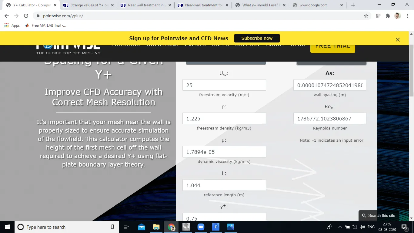
• select first cell thickness based on y+ for that online calculater availablr for y+ calculation. for example as given below for y+ 0.75

• Here we also need to refined inner inclosure mesh element with different case (100 mm , 75 mm , 50 mm..)
• tyre of car body where mesh element size taken as as 5 mm .

• 
• give name selection in the geometry. and proceed with solution part .

3). Solving .

• select the steady state condition and pressure based solver as mach number in case 0.3 incompressible flow .
• To avoid floating point ( high fluctuation in residual ) add underrelaxation factor of pressure and momentum from solution control
• boundary condition
  • inlet : 25 m/s
  • outlet : Zero Guage pressure at o/L
  • car- wall : stationary wall & No slip condition
• select model k-w SST model
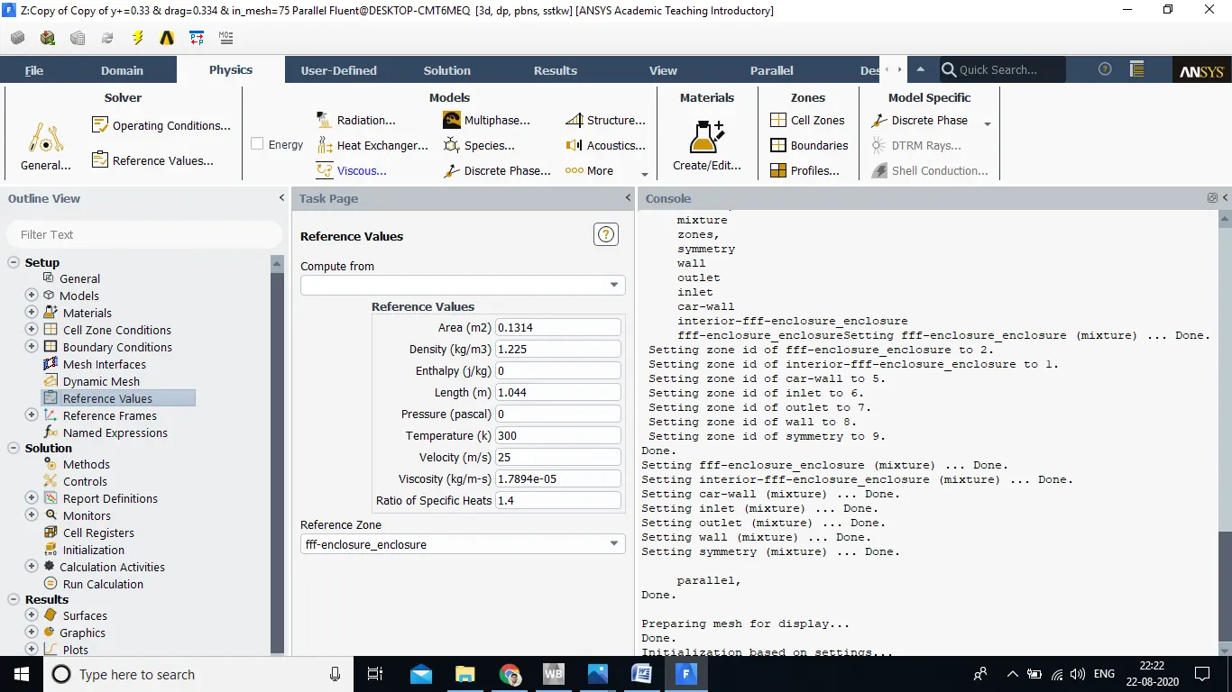
• set appropriate reference value
• 
• intialize the solution hit the calculate button

4). post -processing .

• obtain velocity and pressure contour .
• verify whether wall y+ is in range once it reach to steady state condition.
• obtain vector and steamline plot around the body.

CASE-1 : BASE LINE SETUP ( DEFAULT)

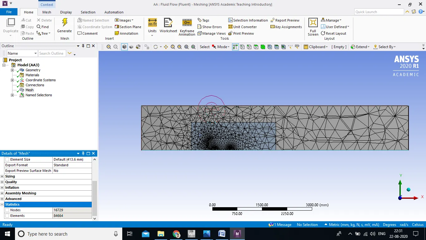
• size. of element : 413.6 mm (overall)
• Number of element : 84864

• 

• Residual plot

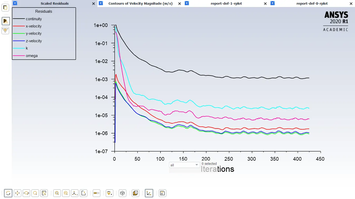
• Residual plot has achieved creteria of 1e-3 and it has got steady condition .

• • Drag and Lift plot

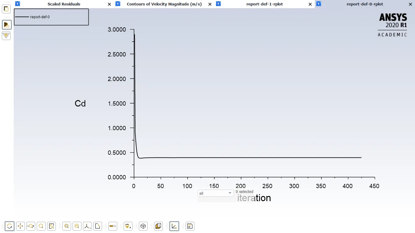
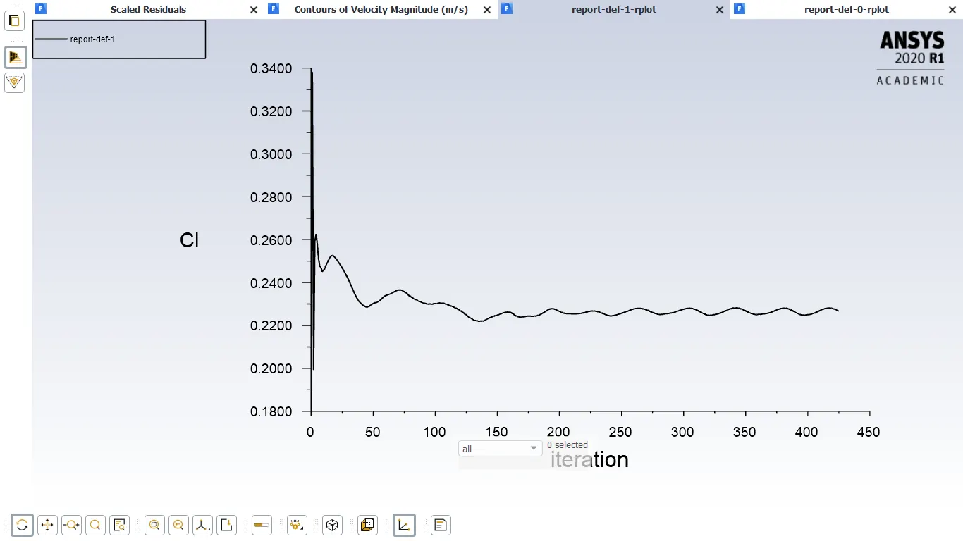
• For above plot Drag co-coefficient value is = 0.396 & lift co-efficient value is = 0.22

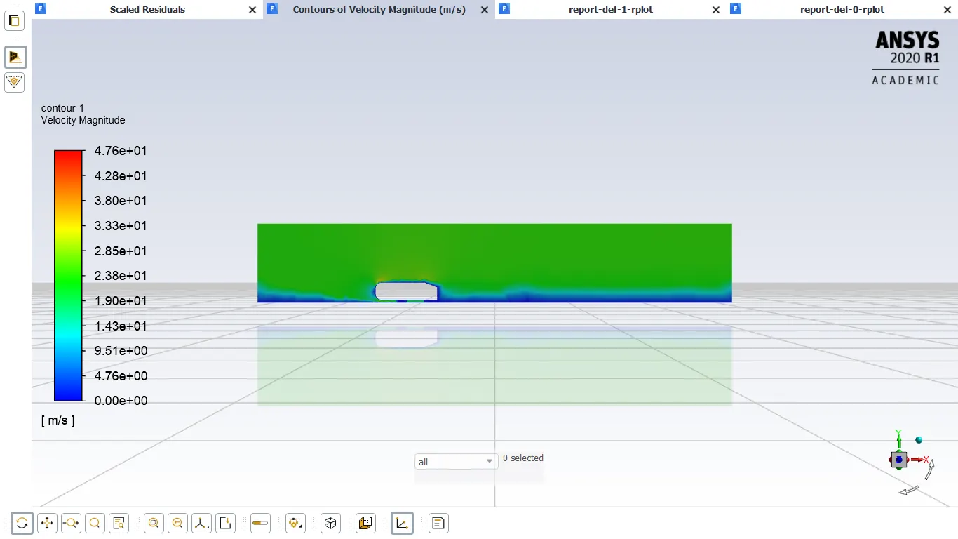
• • velocity contour plot

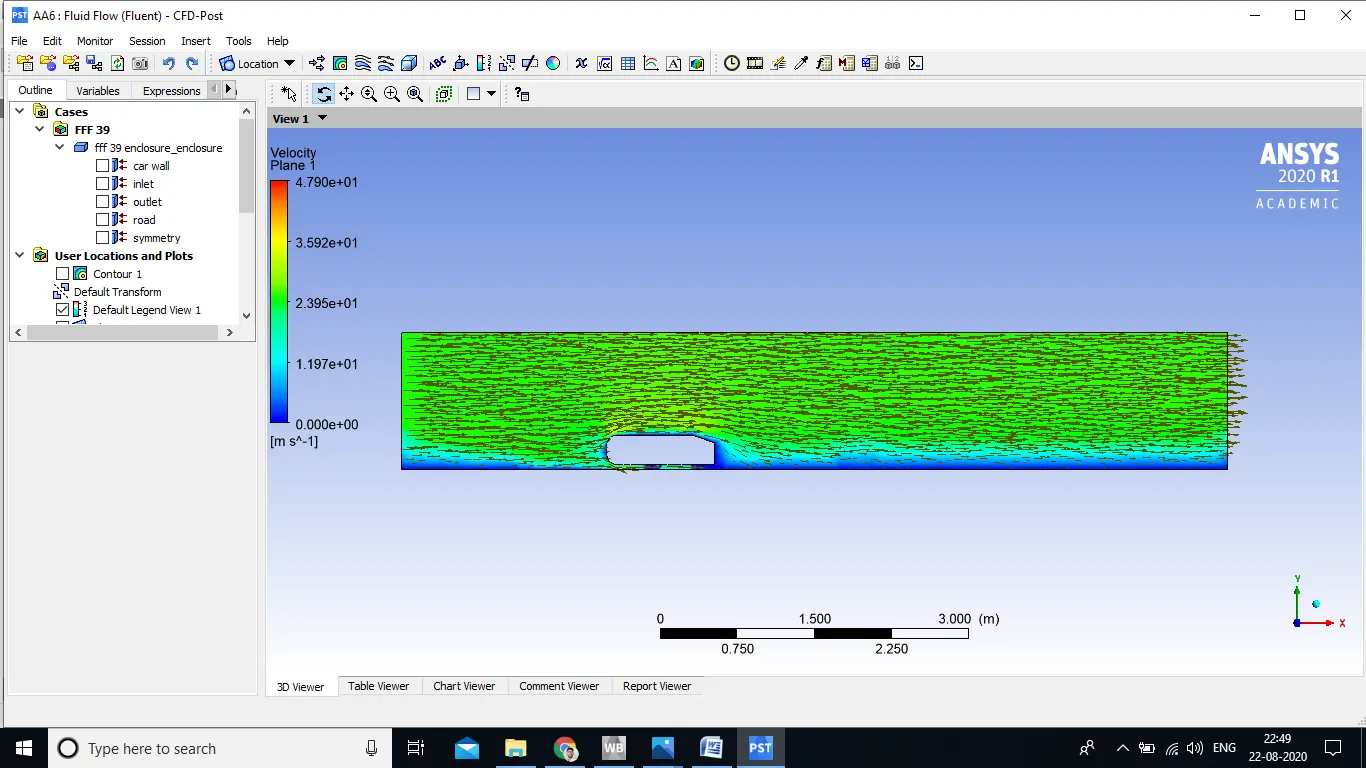
• • vector plot at plane(xy)

CASE-2 :

• size. of element ( outer enclosure ) : 100 mm
• size. of element ( inner enclosure ) : 100 mm
• first layer thickness : 3.5e-3 mm ( based on y+=0.33) & no. of inflation layer =10
• No, of element : 138288

• Residual plot

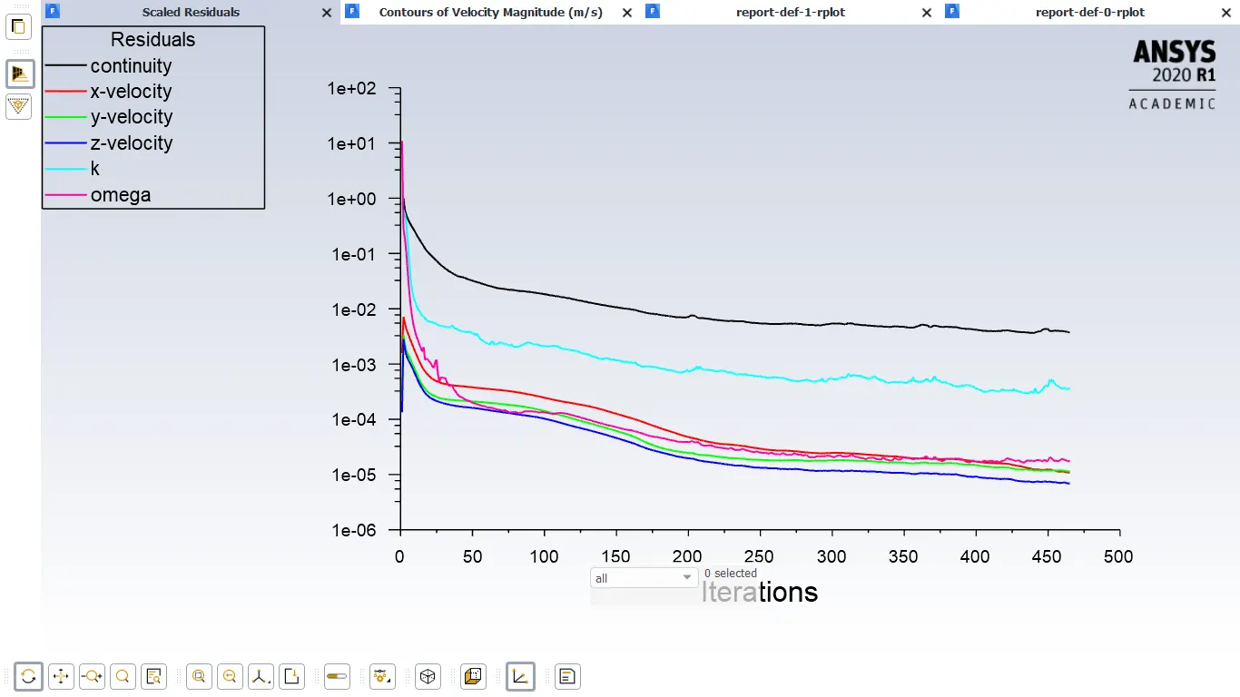
• Residual plot has achieved creteria of 1e-3 and it has got steady condition .

• • Drag and Lift plot

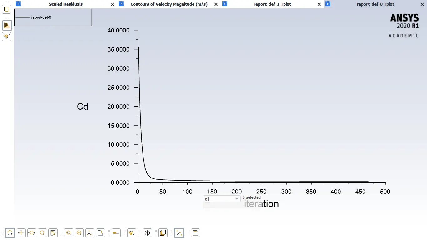
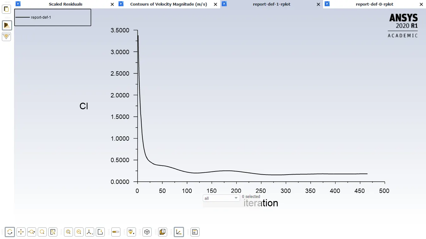
• For above plot Drag co-coefficient value is = 0.396 & lift co-efficient value is = 0.22

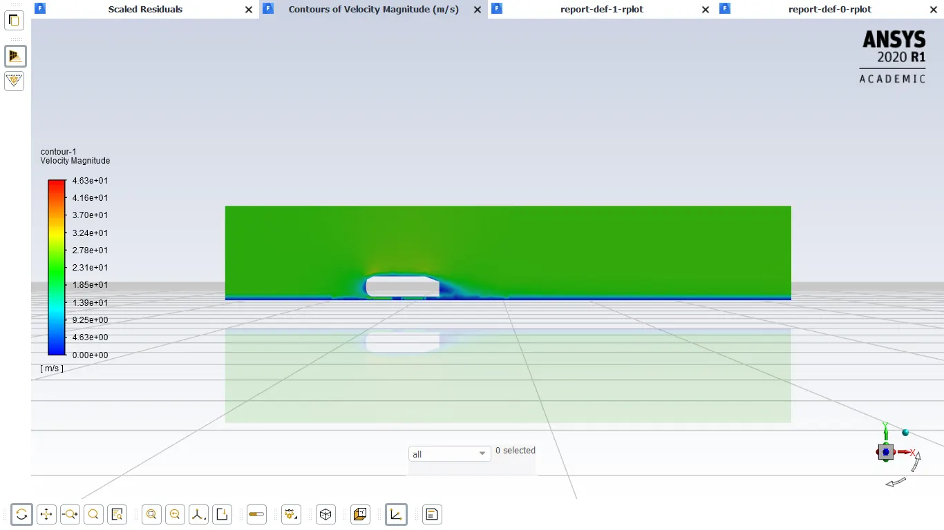
• • velocity contour plot

CASE-1 :

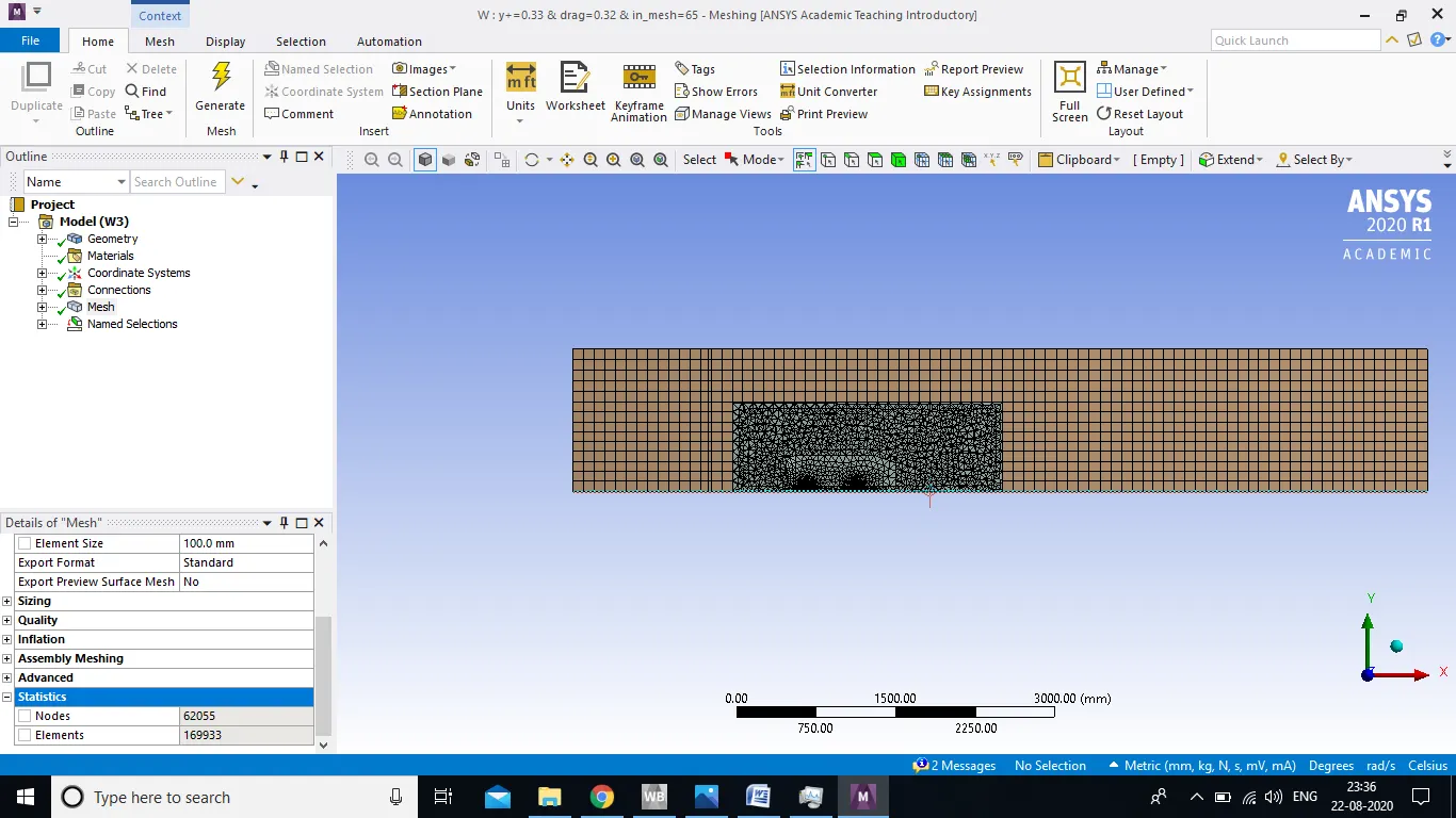
• size. of element ( outer enclosure ) : 100 mm
• size. of element ( inner enclosure ) : 65 mm
• first layer thickness : 3.5e-3 mm ( based on y+=0.33) & no. of inflation layer =10
• No, of element : 169399

• Residual plot

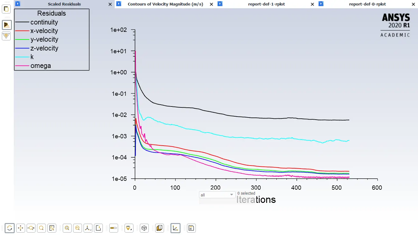
• Residual plot has achieved creteria of 1e-3 and it has got steady condition .

• • Drag and Lift plot

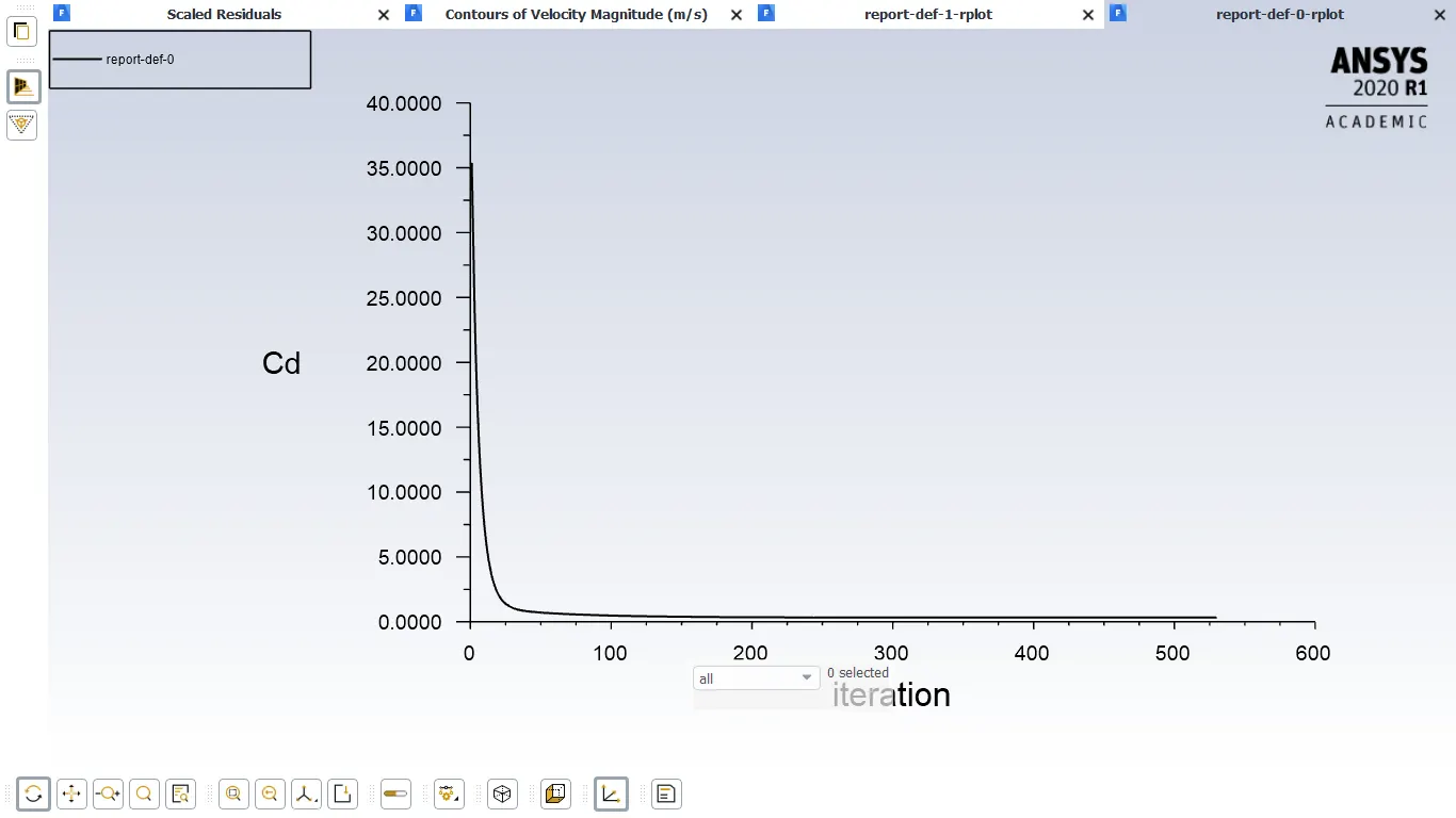
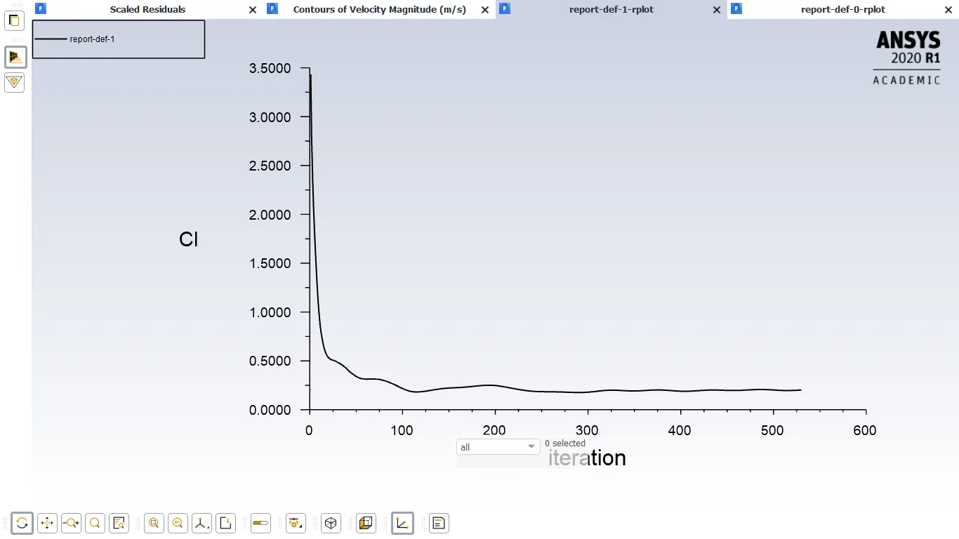
• For above plot Drag co-coefficient value is = 0.336 & lift co-efficient value is = 0.20

• • velocity contour plot

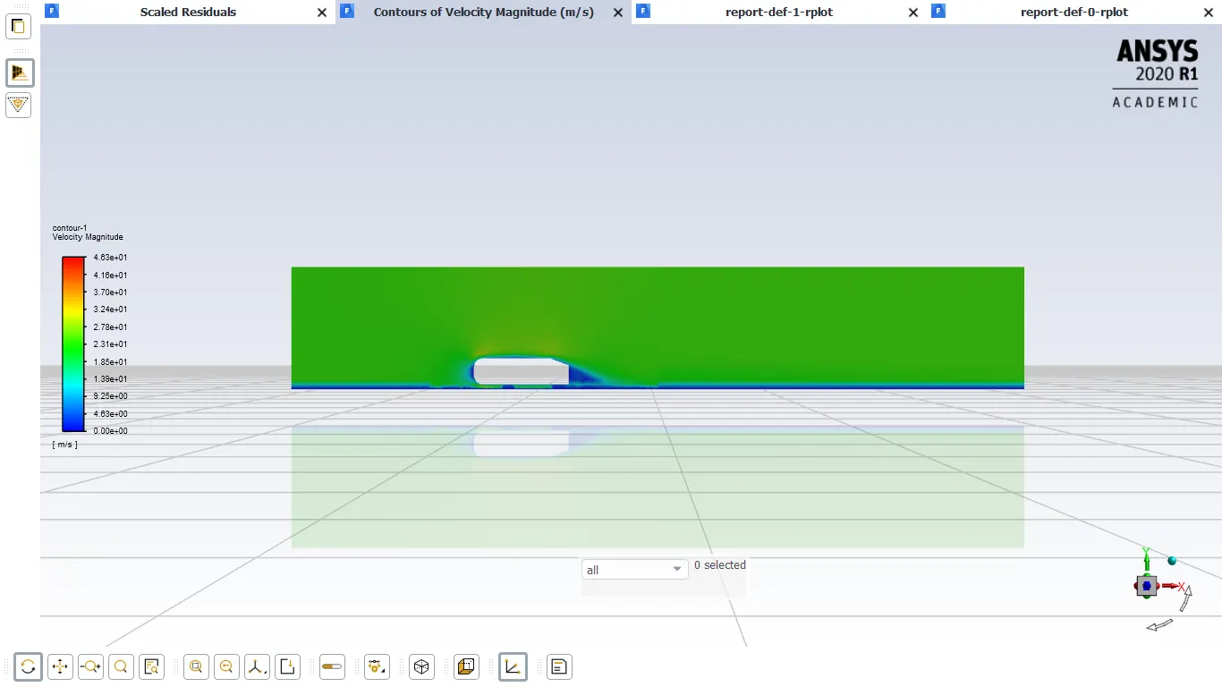
• • vector contour plot

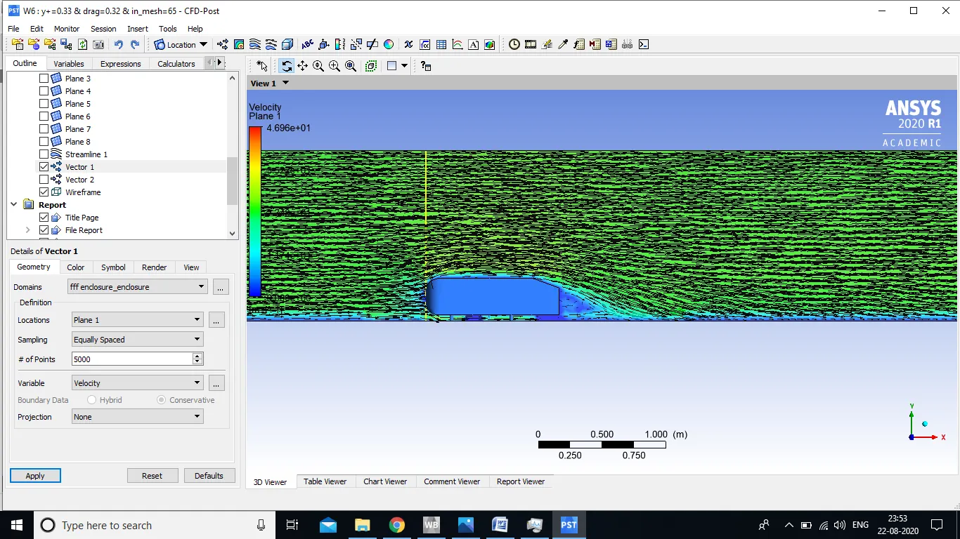
• • streamline plot at rear of body (in x direction at 2.0 m , 1.4m , 1.1 m)

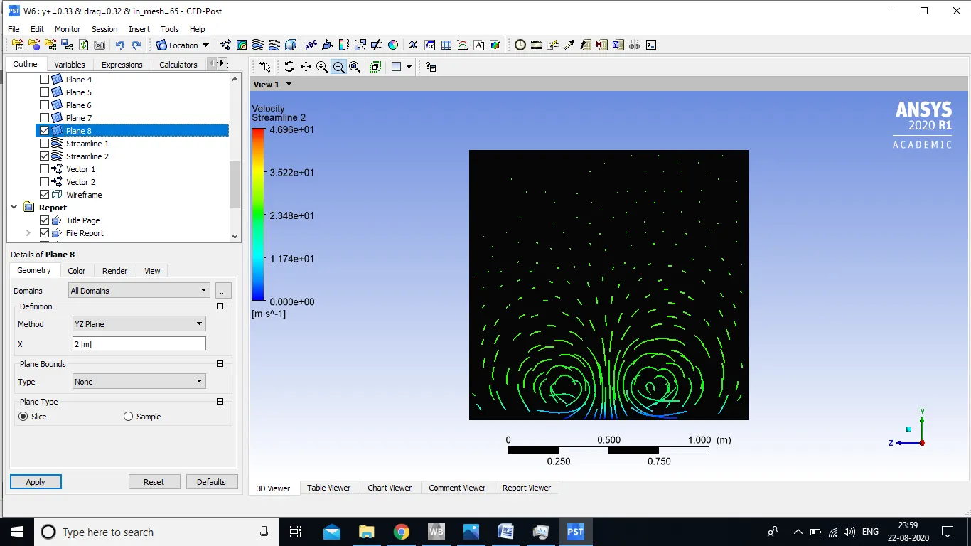
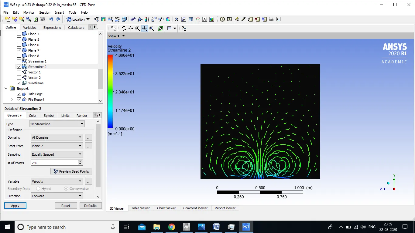
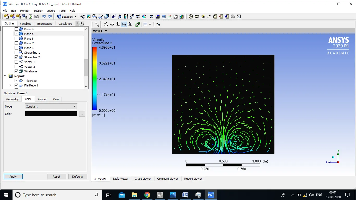
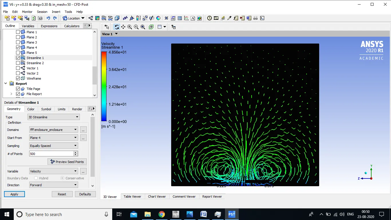
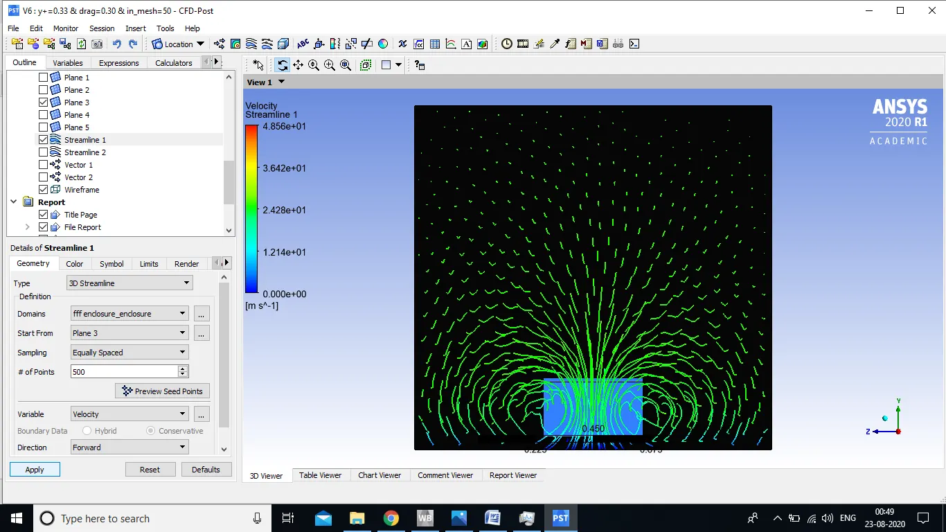
• from above plot of streamline as we go far from stramline seems to more far distributed and for plane close to body 1.1m where streamline is more denser.

• velocity plot at different location behind body (1.1m , 1.2m ,1.4m in x direction)

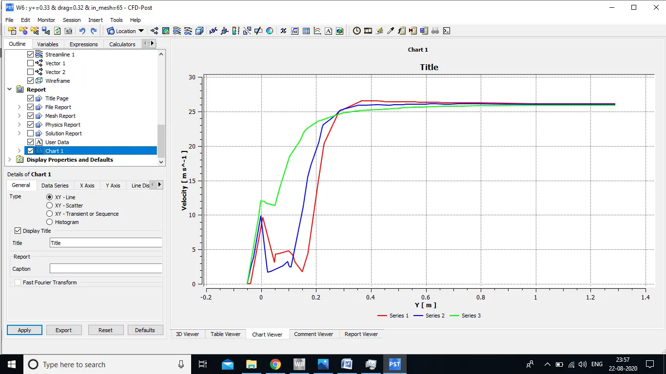
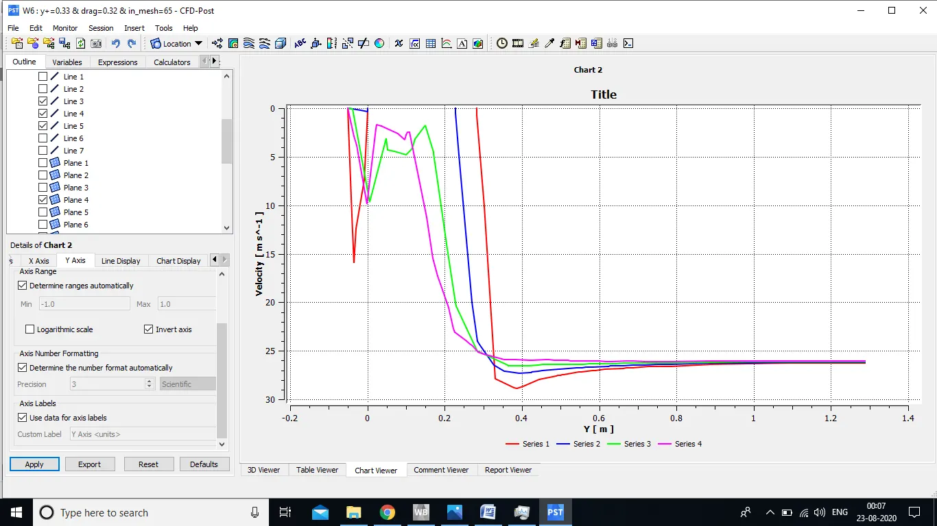
• comparision of velocity plot at front & behind body (0.85 & 1m in front of car and 1.1m & 1.2m in rear direction)

CASE-1 : BASE LINE SETUP ( DEFAULT)

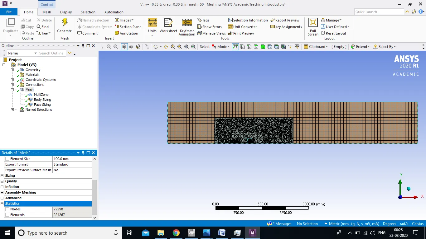
• • size. of element ( outer enclosure ) : 100 mm
  • size. of element ( inner enclosure ) : 50 mm
  • first layer thickness : 3.5e-3 mm ( based on y+=0.33) & no. of inflation layer =10
  • No, of element : 224267

  

• Residual plot

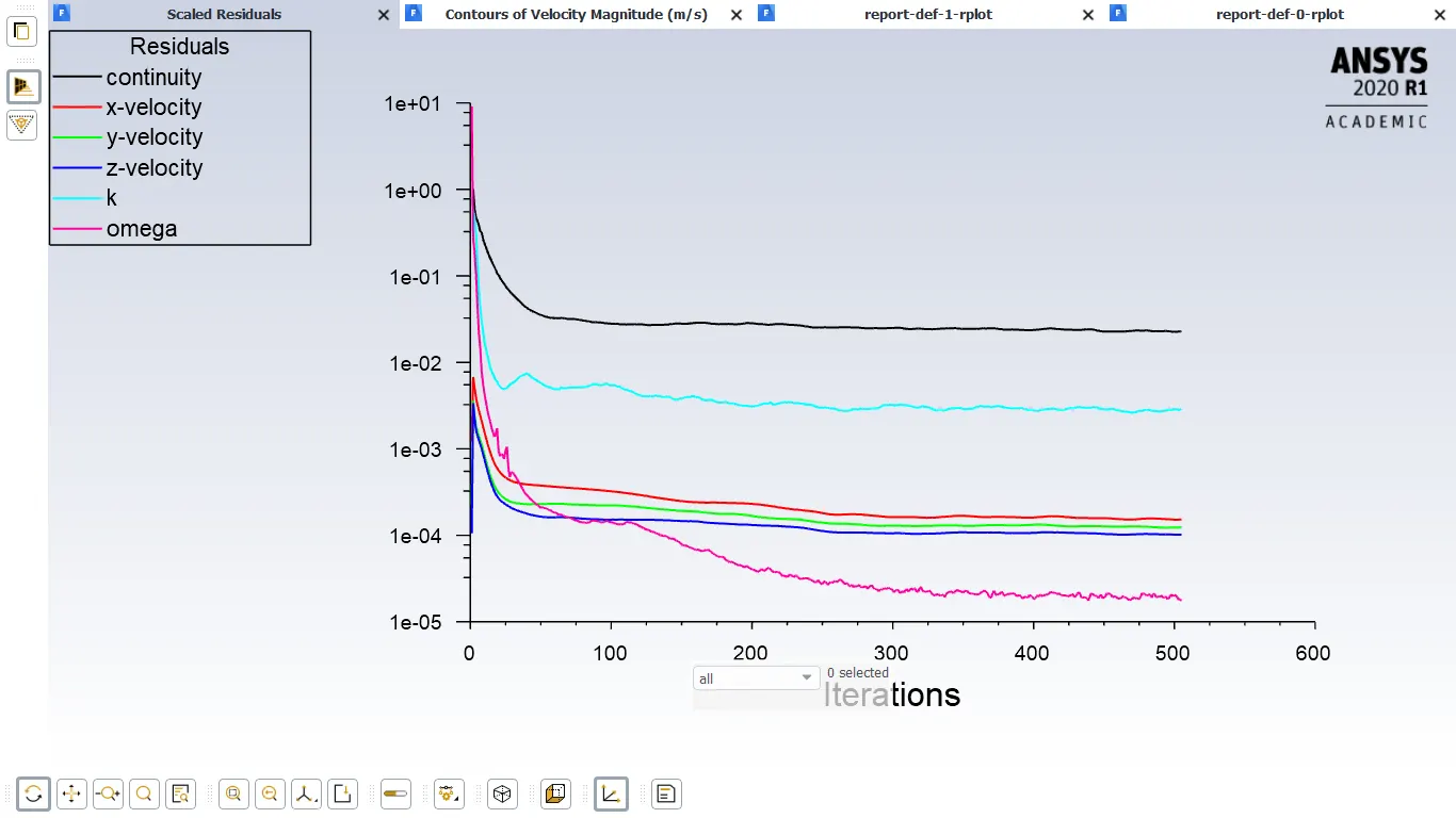
• Residual plot has achieved creteria of 1e-3 and it has got steady condition .

• • Drag and Lift plot

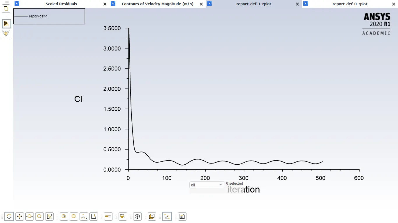
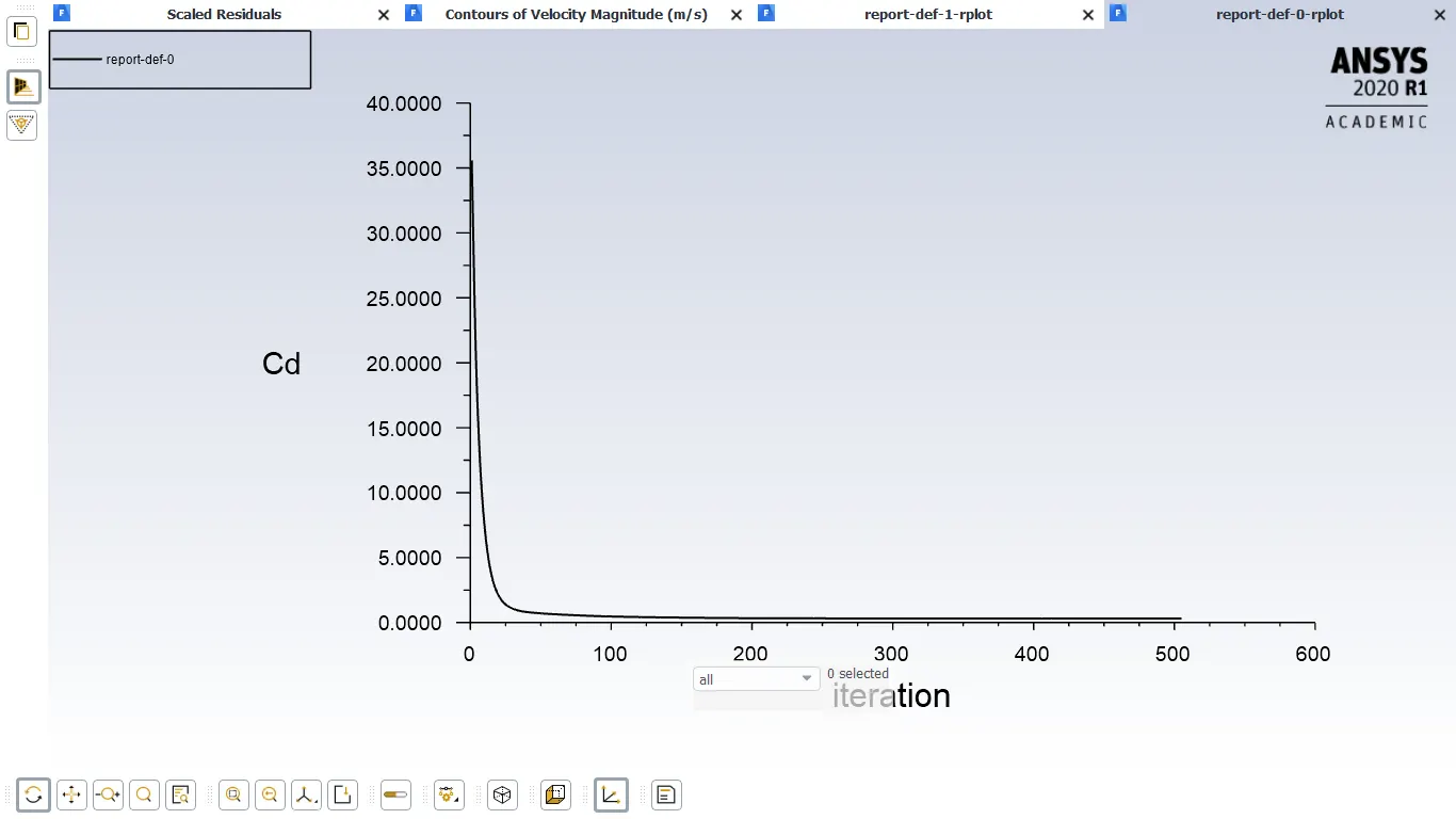
• For above plot Drag co-coefficient value is = 0.304 & lift co-efficient value is = 0.18

• • velocity contour plot
• 

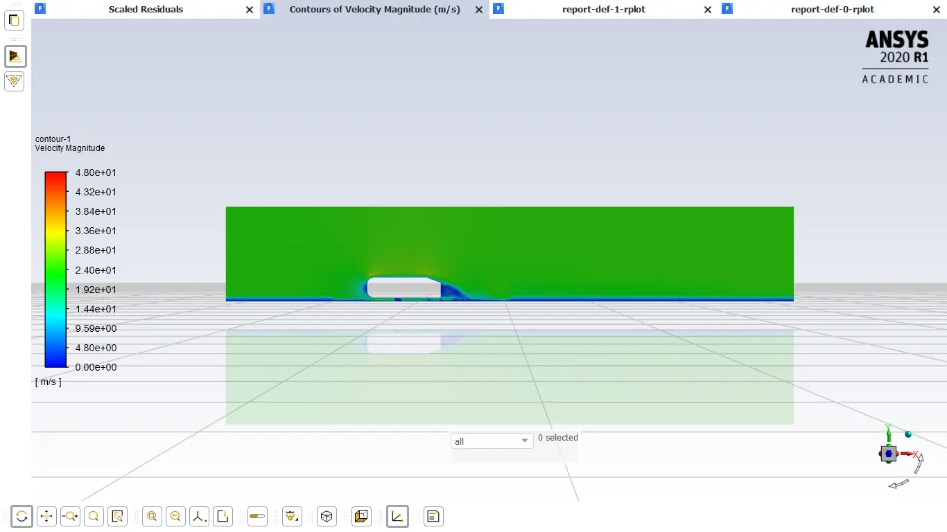
• • vector contour plot

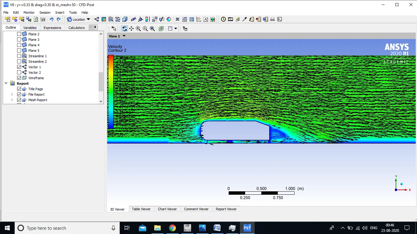
• • streamline plot at rear of body (in x direction at 2.0 m , 1.4m , 1.1 m)

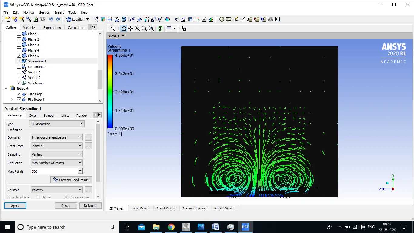
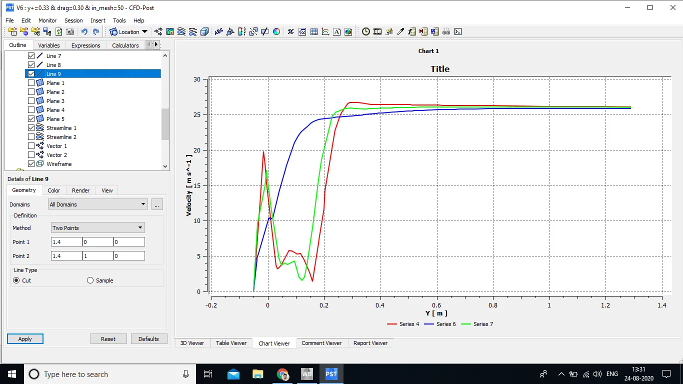
• • velocity plot at different location behind body (1.1m , 1.2m ,1.4m in x direction)

• • comparision of velocity plot at front & behind body (0.85 & 1m in front of car and 1.1m & 1.2m in rear direction)

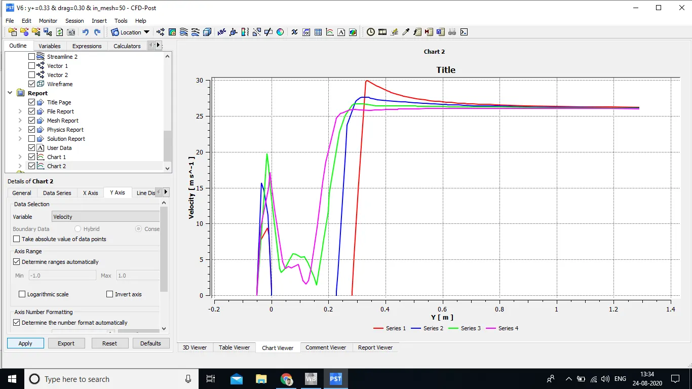
• where red and blue colour plot indicates velocity for front side of body and magenta and green colour indicates plot behind the body
• its can cleary visible from that for behind body as we take line more far from body rear side pressure drop to near about zero because of recirculation region.

the reason for the negative pressure in the wake region. :

• when the vehicle is moving at high velocity no. of molecules of air got deaccelarated because of influence of boundary layer where zero shear stress condition is imposed and thus when the air hits on the front part of body because of zero velocity and thus creates high pressure on the front part of vehicle because at the part of body molecule starts to compressing.
• as air molecules with particular streanline moves ahead along the body its fluid imposes the pressure on the boundary layer because of less pressure than front of vehicle and when the air reaches to rear part of body fluid get deatched due to unfavourable pressure gradient and fluid start to moving around the body creates the circulation region which called as wake.
• when the air get seperated at the rear its creates the low pressure region behind the body known as wakw .
• effect of wake , size of wake & position of wake on body can produce significant effect on drag and thus on car performance too.