ODE to describe the transient behavior of a Pendulum

The equation given is a second order ODE, i.e.,

`(d^2theta)/dt^2 + b/m (d theta)/dt + g/L sin theta = 0`

hence this equation can be written as,

`(d^2 theta)/dt^2 = -b/m (d theta)/dt - g/L sin theta` ...eqn(1)

This equation is converted in 1st order ODE.

`theta_1 = theta(1)` --> this term indicates displacement ...eqn(2)

`dot theta = theta (2)` -->this term indicates velocity ...eqn(3)

`ddot theta = (d dot theta)/dt = (d^2 theta)/dt^2` ...eqn(4)

now substituting equations (2), (3), and (4) in equation (1), we have

`ddot theta = - b/m theta_2 - g/L sin(theta_1)` ...eqn(5)

from equations (3) and (5), we have

`dot theta = theta (2)`

`ddot theta = - b/m theta_2 - g/L sin(theta_1)`

we can observe that second order differential equation into 2 1st order ODE.

This ODE is written as a function that generates two outputs. The 1st column represents the displacement and the second column represents the velocity. These values are plotted on a graph with the x-axis representing the time.

The boundary conditions assigned to the problem are:

Length L = 1m

Mass m = 1kg

g = 9.81 m/s^2

damping coefficient b = 0.5 [higher value of damping coefficient is used because we can observe a smooth graph with better damping]

MATLAB Code:

% Main Body of the program 

clear all 
close all 
clc 

%Data of ODE 
%Acceleration due to gravity 
g = 9.81; 

%Length of pendulum 
L = 1; 

%Mass of pendulum 
m = 1; 

%damping coeffient 
b = 0.5; 

%Initial condtions 
theta0 = [0 3]; 
time = linspace(0,30,200); 

%Solving using ODE45 
[t, solution] = ode45(@(t,theta) discrtitzing_function(t, theta, g, L, m, b), time, theta0); 

%plotting 
figure(1) 
plot(t,solution(:, 1)) 
axis([0 20 -4 4]); 
hold on 
plot(t,solution(:, 2),'g'); 
grid on 
xlabel('Time'); 
ylabel('Amplitude'); 
legend('Angular Displacement', 'Angular Velocity'); 

%Creating animation for pendulum 
theta = solution(:,1); 
ct = 1; 
for i = 1:length(theta) 
    THETA = theta(i); 
    
    %Initializing starting point for pendulum 
    x0 = 0; 
    y0 = 0; 
    
    %Displacement of the pendulum 
    x1 = L*sin(THETA); 
    y1 = -L*cos(THETA); 
    
    figure (2); 
    %Plotting string 
    plot([x0 x1], [y0 y1],'color', 'black'); 
    grid on 
    hold on 
    
    %Plotting pendulum bob
    plot(x1,y1,'o','markersize',20,'color','r','MarkerFaceColor','r'); 
    hold off 
    
    axis([-1 1 -1.5 0]); 
    pause(0.003); 
    mov(ct) = getframe(gcf); 
    ct = ct+1; 
end 

%creating a movie 
movie(mov); 
videofile = VideoWriter('Pendulum.avi', 'Uncompressed avi'); 
open(videofile) 
writeVideo(videofile,mov) 
close(videofile)

% Function to calculate time and theta

function out = discrtitzing_function(t, theta, g, L, m, b);
theta1 = theta(1);
theta2 = theta(2);
theta_dot = theta2;
theta_double_dot = -(b/m)*theta2-(g/L)*theta1;
out = [theta_dot; theta_double_dot];
end

https://www.youtube.com/watch?v=dOUECUwnsR0

The video depicts the oscillation of the pendulum having a string length of 1m, the mass of 1kg, and b as 0.5.

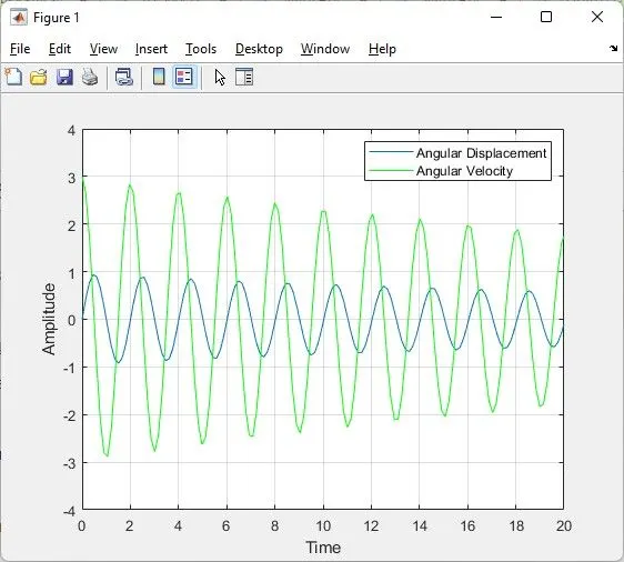
Fig 1. Damping obtained when b = 0.05

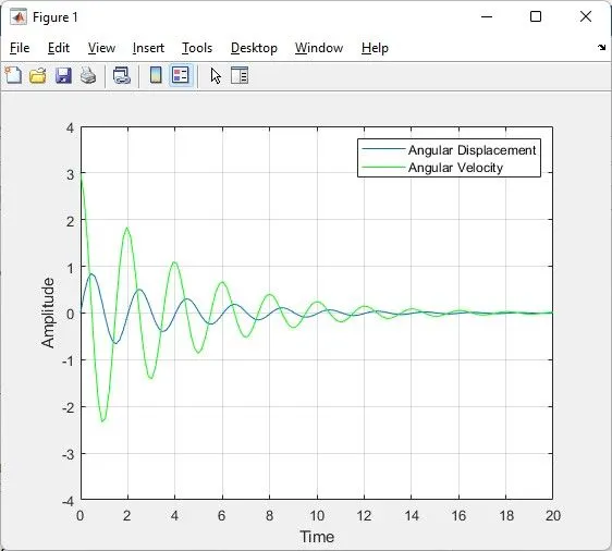
Fig 2. Damping obtained when b = 0.5

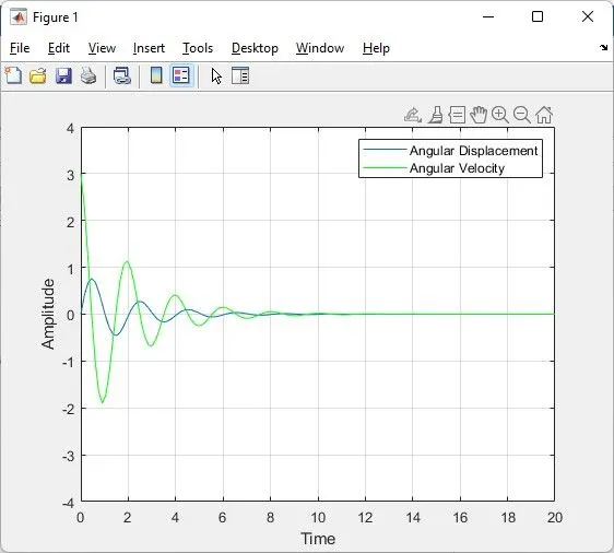
Fig 3. Damping obtained when b = 1

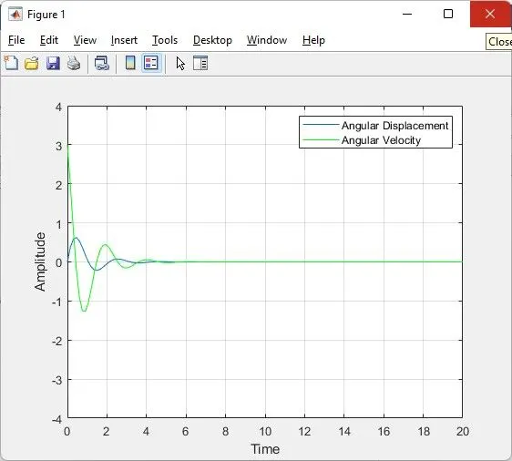
Fig 4. Damping obtained when b = 2

From the above graph, we can clearly observe that as the coefficient of damping(b) increases, the pendulum tries to attain its original position quickly.