SIMULATING AIR STANDARD CYCLE

AIM: To Simulate an Air standard cycle using MATLAB.

OBJECTIVE: The Objective of this project is to write a program in the MATLAB and execute it to get the desired plots.

THEORY:

The air standard cycle is a part of Thermodynamics cycle. which includes various cycles like OTTO CYCLE, CARNOT CYCLE, and STIRLING CYCLE, BRAYTON CYCLE and so on. In this cycle the addition of heat takes place externally, Hence they are also called the external combustion engines. The Most commonly used pratical engines used in our day-to-day life are internal combustion engines for our vehicles , motor cycles, construction machineries etc.

DEFINATIONS:

• THERMODYNAMICS: Thermodynamics is a branch of physics that deals with heat and temperature, and their relation to energy, work, radiation, and properties of matter.

LAWS OF THERMODYNAMIS:

ZEROTH OF THERMODYNAMICS: The zeroth law of thermodynamics states that if two systems are both in thermal equilibrium with a third system, then the first two systems are also in thermal equilibrium with each other.

1ST LAW OF THERMODYNAMICS: The first law of thermodynamics is the physical law which states that the total energy of a system and its surroundings remain constant. The law is also known as the law of conservation of energy, which states energy can transform from one form into another, but can neither be created nor destroyed within an isolated system.

2ND LAW OF THERMODYNAMICS: The second law of thermodynamics says that the entropy of any isolated system always increases. Isolated systems spontaneously evolve towards thermal equilibrium—the state of maximum entropy of the system.

3RD LAW OF THERMODYNAMICS: The Third law of thermodynamics states that as the temperature of the system approches absolute zero, its entropy becomes constant, or change in the entropy is zero. The third law of thermodynamics predicts the properties of a system and behaviour of entropy in a unique environment known as absolute temperature

OTTO-CYCLE:

P-V DIAGRAM

An Otto cycle is an idealized thermodynamics cycle that describes the functioning of a typical spark ignition piston engine. It is the thermodynamic cycle most commonly found in automobile engines.

The role and the process of the above P-V diagram as follows:

Process 1-2 = Isotropic Compression

Process 2-3 = Constant Volume heat addition

Process 3-4 = Isotropic Expansion

Process 4-2 = Constant volume heat rejection

CYCLE ANALYSIS:

• In the process 1–2 the piston does work on the gas and in process
• In the process 3–4 the gas does work on the piston during those isentropic compression and expansion processes, respectively.
• In the Processes 2–3 and 4–1 are isochoric processes; heat is transferred into the system from 2—3 and out of the system from 4—1 but no work is done on the system or extracted from the system during those processes.
• No work is done during an isochoric (constant volume) process because addition or removal of work from a system requires the movement of the boundaries of the system; hence, as the cylinder volume does not change, no shaft work is added to or removed from the system.

These are the values obtained from the work space after the execution of the program.

THERMAL EFFICIENCY:

From the above data given

Let, The starting point is the general expression for the thermal efficiency of a cycle:

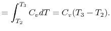
The convention, as previously, is that heat exchange is positive if heat is flowing into the system or engine, so is negative. The heat absorbed occurs during combustion when the spark occurs, roughly at constant volume. The heat absorbed can be related to the temperature change from state 2 to state 3 as:

The heat rejected is given by (for a perfect gas with constant specific heats)

Substituting the expressions for the heat absorbed and rejected in the expression for thermal efficiency yields

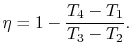
We can simplify the above expression using the fact that the processes from 1 to 2 and from 3 to 4 are isentropic:

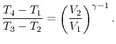
The quantity is called the compression ratio. In terms of compression ratio, the efficiency of an ideal Otto cycle is:

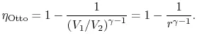
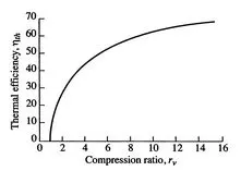
The ideal Otto cycle efficiency is shown as a function of the compression ratio . As the compression ratio, , increases, increases, but so does . If is too high, the mixture will ignite without a spark at the wrong location in the cycle.

PISTON KINEMATICS OF ENGINE:

where,

IV – intake valve

EV – exhaust valve

TDC – top dead center

BDC – bottom dead center

B – cylinder bore

S – piston stroke

r – connecting rod length

a – crank radius (offset)

x – distance between the crank axis and the piston pin axis

θ – crank angle

V_d – displaced (swept) volume

V_c – clearance volume

An internal combustionengine is a heat engine whichconverts chemical energyfrom fuel into mechanical
energy of the crank-slidermechanism.Duringcombustion process, the fuelis burnt in the combustionchamber (i.e. the spacebetween the piston and thetop of the cylinder)

The combustion process raises the gas temperature andpressure hence pushes the piston along the negative xaxis. This linear motion is converted into rotational motion via
crank-slider mechanism which consists of wrist pin,connecting rod, crank pin, crank and main pin. The
torque resulting from the rotational motion of the crank istransferred to propel vehicles or other devices.

PROGRAM IN THE MATLAB FOR PISTON KINEMATICS:

clear all
close all
clc
% inputs
gamma= 1.4
t3= 2300

% state variables
p1= 101325
t1= 500

% Engine geometric parameters
bore = 0.1;
stroke= 0.1;
con_rod= 0.15;
cr= 12;

% calculating the swept volume and the clerance volume 
v_swept = (pi/4)*bore^2*stroke;
v_clerance = v_swept/(cr-1);
v1= v_swept+v_clerance
v2= v_clerance

%state variables at state point 2
%p2v2^gamma=p1v1^gamma
%p2= p1*(v1/v2)^gamma=p1*cr^gamma
%p2=p1*(v1/v2)^gamma= p1*cr^gamma
p2= p1*cr^gamma;

% p1v1/t1 p2v2/t2 | t2= p2*v2*t1?(p1*v1)
t2= p2*v2*t1/(p1*v1);
constant_c= p1*v1^gamma;
v_compression = engine_kinematics1(bore,stroke,con_rod,cr,180,0);
p_compression= constant_c./v_compression.^gamma;
% state variable at state point 3
v3 = v2

% p3v3/t3= p2v2/t2 | p3=p2*t3/t2
p3=p2*t3/t2

constant_c= p3*v3^gamma;
v_expansion = engine_kinematics1(bore,stroke,con_rod,cr,0,180);
p_expansion= constant_c./v_expansion.^gamma;

%  state variable at state point 4
v4 = v1

% p3v3^gamma=p4v4^gamma | p4=p3(v3/v4)^gamma
p4= p3*(v3/v4)^gamma


figure(1)
hold on
plot(v1,p1,'*','color','r')
plot(v_compression,p_compression)
plot(v2,p2,'*','color','y')
plot(v3,p3,'*','color','b')
plot(v_expansion,p_expansion)
plot(v4,p4,'*','color','g')

ERRORS IN THE CODE:

CODE EXPLANATION:

In the above program by taking the inputs and state variables of the engine geometric parameters. The values are given in the programming through different terms as Term 1,2,3 and coded for the State varaibles of P1,V1,T1, and P2,V2,T2, and also fro P3,V3,T3 respectively and finally by using the plotting command for compression and expansion with four different colours to visible clearly. By completion of programming plottings are as below. Better explained in programming code.

CONCLUSION: By calculating the swept volume and the clerance volume,with the engine geometric parameters and their inputs.The state variables are obtained to plot the P-V Diagram and the Thermal efficiency of the engine.

RESULT: Simulation of Air standard cycle is obtained by executing a program in MATLAB.