Global maxima of a Stalagmite function using Genetic Algorithm
Objective:
The main objective of this project is to write a code in MATLAB to optimise the stalagmite function and find the global maxima of the function. Also to understand the concept of Genetic algorithm and the syntax for ga (genetic algorithm) in matlab program.
Genetic Algorithm:
A genetic algorithm is a search heuristic that is inspired by Charles Darwin’s theory of natural evolution.It is frequently used to find optimal or near-optimal solutions to difficult problems which otherwise would take a lifetime to solve. It is frequently used to solve optimization problems, in research, and in machine learning.
Genetic algorithms are a specific approach to optimization problems that can estimate known solutions and simulate evolutionary behavior in complex systems.
Algorithm in Matlab to find Global minima:
A genetic algorithm (GA) is a method for solving both constrained and unconstrained optimization problems based on a natural selection process that mimics biological evolution. The algorithm repeatedly modifies a population of individual solutions. At each step, the genetic algorithm randomly selects individuals from the current population and uses them as parents to produce the children for the next generation. Over successive generations, the population "evolves" toward an optimal solution.
You can apply the genetic algorithm to solve problems that are not well suited for standard optimization algorithms, including problems in which the objective function is discontinuous, nondifferentiable, stochastic, or highly nonlinear.
Optimization:
Optimization is the process of making something better. In any process, we have a set of inputs and a set of outputs as shown in the following figure.
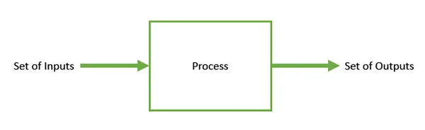
Optimization refers to finding the values of inputs in such a way that we get the “best” output values. The definition of “best” varies from problem to problem, but in mathematical terms, it refers to maximizing or minimizing one or more objective functions, by varying the input parameters.
The set of all possible solutions or values which the inputs can take make up the search space. In this search space, lies a point or a set of points which gives the optimal solution. The aim of optimization is to find that point or set of points in the search space.
Basic structure:
The basic structure of a GA is as follows −
We start with an initial population (which may be generated at random or seeded by other heuristics), select parents from this population for mating. Apply crossover and mutation operators on the parents to generate new off-springs. And finally these off-springs replace the existing individuals in the population and the process repeats. In this way genetic algorithms actually try to mimic the human evolution to some extent.
Each of the following steps are covered as a separate chapter later in this tutorial.
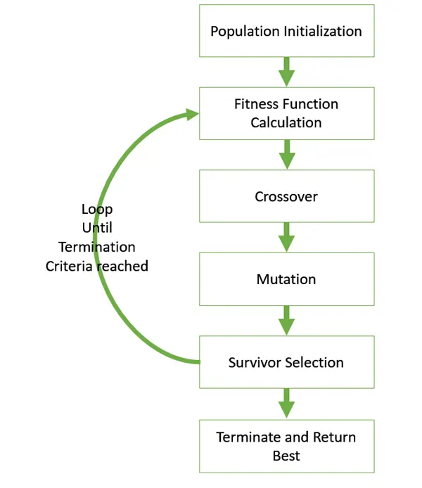
Outline of the Algorithm
The following outline summarizes how the genetic algorithm works:
-
The algorithm begins by creating a random initial population.
-
The algorithm then creates a sequence of new populations. At each step, the algorithm uses the individuals in the current generation to create the next population. To create the new population, the algorithm performs the following steps:
-
Scores each member of the current population by computing its fitness value. These values are called the raw fitness scores.
-
Scales the raw fitness scores to convert them into a more usable range of values. These scaled values are called expectation values.
-
Selects members, called parents, based on their expectation.
-
Some of the individuals in the current population that have lower fitness are chosen as elite. These elite individuals are passed to the next population.
-
Produces children from the parents. Children are produced either by making random changes to a single parent—mutation—or by combining the vector entries of a pair of parents—crossover.
-
Replaces the current population with the children to form the next generation.
-
-
The algorithm stops when one of the stopping criteria is met.
Initial Population:
The algorithm begins by creating a random initial population, as shown in the following figure.
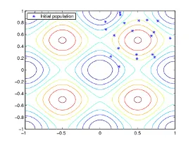
In this example, the initial population contains
20individuals. Note that all the individuals in the initial population lie in the upper-right quadrant of the picture, that is, their coordinates lie between 0 and 1. For this example, the Initial range in the Population options is[0;1].If you know approximately where the minimal point for a function lies, you should set Initial range so that the point lies near the middle of that range. For example, if you believe that the minimal point for Rastrigin's function is near the point
[0 0], you could set Initial range to be[-1;1]. However, as this example shows, the genetic algorithm can find the minimum even with a less than optimal choice for Initial range.Creating the Next Generation:
At each step, the genetic algorithm uses the current population to create the children that make up the next generation. The algorithm selects a group of individuals in the current population, called parents, who contribute their genes—the entries of their vectors—to their children. The algorithm usually selects individuals that have better fitness values as parents. You can specify the function that the algorithm uses to select the parents in the Selection function field in the Selection options.
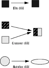
The genetic algorithm creates three types of children for the next generation:
-
Eliteare the individuals in the current generation with the best fitness values. These individuals automatically survive to the next generation.
-
Crossover are created by combining the vectors of a pair of parents.
-
Mutation children are created by introducing random changes, or mutations, to a single parent.
The following schematic diagram illustrates the three types of children.
Mutation and Crossover explains how to specify the number of children of each type that the algorithm generates and the functions it uses to perform crossover and mutation.
The following sections explain how the algorithm creates crossover and mutation children.
Crossover Children
The algorithm creates crossover children by combining pairs of parents in the current population. At each coordinate of the child vector, the default crossover function randomly selects an entry, or gene, at the same coordinate from one of the two parents and assigns it to the child. For problems with linear constraints, the default crossover function creates the child as a random weighted average of the parents.
Mutation Children
The algorithm creates mutation children by randomly changing the genes of individual parents. By default, for unconstrained problems the algorithm adds a random vector from a Gaussian distribution to the parent. For bounded or linearly constrained problems, the child remains feasible.
The following figure shows the children of the initial population, that is, the population at the second generation, and indicates whether they are elite, crossover, or mutation children.
-
Selection:
The selection function chooses parents for the next generation based on their scaled values from the fitness scaling function. The scaled fitness values are called the expectation values. An individual can be selected more than once as a parent, in which case it contributes its genes to more than one child. The default selection option, Stochastic uniform, lays out a line in which each parent corresponds to a section of the line of length proportional to its scaled value. The algorithm moves along the line in steps of equal size. At each step, the algorithm allocates a parent from the section it lands on.
A more deterministic selection option is Remainder, which performs two steps:
-
In the first step, the function selects parents deterministically according to the integer part of the scaled value for each individual. For example, if an individual's scaled value is 2.3, the function selects that individual twice as a parent.
-
In the second step, the selection function selects additional parents using the fractional parts of the scaled values, as in stochastic uniform selection. The function lays out a line in sections, whose lengths are proportional to the fractional part of the scaled value of the individuals, and moves along the line in equal steps to select the parents.
Note that if the fractional parts of the scaled values all equal 0, as can occur using
Topscaling, the selection is entirely deterministic.
Reproduction Options:
Reproduction options control how the genetic algorithm creates the next generation. The options are
-
Elite count — The number of individuals with the best fitness values in the current generation that are guaranteed to survive to the next generation. These individuals are called elite children. The default value of Elite count is 5% of the population size, rounded up.
When Elite count is at least 1, the best fitness value can only decrease from one generation to the next. This is what you want to happen, since the genetic algorithm minimizes the fitness function. Setting Elite count to a high value causes the fittest individuals to dominate the population, which can make the search less effective.
-
Crossover fraction — The fraction of individuals in the next generation, other than elite children, that are created by crossover. Setting the Crossover Fraction describes how the value of Crossover fraction affects the performance of the genetic algorithm.
Because elite individuals have already been evaluated, ga does not reevaluate the fitness function of elite individuals during reproduction. This behavior assumes that the fitness function of an individual is not random, but is a deterministic function. To change this behavior, use an output function.
Mutation and Crossover:
The genetic algorithm uses the individuals in the current generation to create the children that make up the next generation. Besides elite children, which correspond to the individuals in the current generation with the best fitness values, the algorithm creates
-
Crossover children by selecting vector entries, or genes, from a pair of individuals in the current generation and combines them to form a child
-
Mutation children by applying random changes to a single individual in the current generation to create a child
Both processes are essential to the genetic algorithm. Crossover enables the algorithm to extract the best genes from different individuals and recombine them into potentially superior children. Mutation adds to the diversity of a population and thereby increases the likelihood that the algorithm will generate individuals with better fitness values.
See Creating the Next Generation for an example of how the genetic algorithm applies mutation and crossover.
You can specify how many of each type of children the algorithm creates as follows:
-
Elite count, in Reproduction options, specifies the number of elite children.
-
Crossover fraction, in Reproduction options, specifies the fraction of the population, other than elite children, that are crossover children.
For example, if the Population size is 20, the Elite count is 2, and the Crossover fraction is 0.8, the numbers of each type of children in the next generation are as follows:
-
There are two elite children.
-
There are 18 individuals other than elite children, so the algorithm rounds 0.8*18 = 14.4 to 14 to get the number of crossover children.
-
The remaining four individuals, other than elite children, are mutation children.
Function used for finding global maxima and minima:
The above function is solved in the matlab program. This function is used as the input for the ga algorithm function.
Let us see the Matlab program for finding the global maxima:
close all
clear all
clc

% Defining the search space
x = linspace(0,0.6,150);
y = linspace(0,0.6,150);

% creating 2 Dimensional mesh
[xx,yy] = meshgrid(x,y);

% Evaluating the stalagmite function
for i = 1:length(xx)
    for j = 1:length(yy)
        input_vector(1) = xx(i,j);
        input_vector(2) = yy(i,j);
        f(i,j) = stalagmite(input_vector);
    end
end

surface(xx,yy,f)
shading interp
xlabel('x value')
ylabel('y value')

[inputs, fval] = ga(@stalagmite,2);
Function code for stalagmite:
The -ve sign is used in the output to plot the graph in inverted position.
function out = stalagmite(input_vector)

f_1 = (sin(5.1*pi*input_vector(1)+0.5)).^6;
f_2 = exp(-4*log(2)*(input_vector(1)-0.0667).^2/(0.64));

f_3 = (sin(5.1*pi*input_vector(2)+0.5)).^6;
f_4 = exp(-4*log(2)*(input_vector(2)-0.0667).^2/(0.64));

out = -(f_1)*(f_2)*(f_3)*(f_4);
end
Plotting Global maxima and minima:
In the below graph we can find the global maximum point, which is in the botton left and minimum point is in the top right.
Program 1:
Here we are running the program under for loop condition with the (num_cases = 50). This command will run the genetic algorithm for 50 iterations. Also we are storing the runtime value with the tic toc command.
close all
clear all
clc

% Declaring input arrays
x = linspace(0,0.6,150);
y = linspace(0,0.6,150);
num_cases = 50; % running the ga 50 times

% creating 2 Dimensional mesh
[xx,yy] = meshgrid(x,y);

% Evaluating the stalagmite function
for i = 1:length(xx)
    for j = 1:length(yy)
        input_vector(1) = xx(i,j);
        input_vector(2) = yy(i,j);
        f(i,j) = stalagmite(input_vector);
    end
end

tic
% study 1 - statistical behaviour
for i = 1:num_cases
    [inputs, fopt(i)] = ga(@stalagmite, 2);
    xopt(i) = inputs(1);
     yopt(i) = inputs(2);
end
study1_time = toc;

% plotting
figure(1)
subplot(2,1,1)
hold on
surfc(x,y,f)
shading interp
plot3(xopt,yopt,fopt,'marker','o','markersize',5,'markerfacecolor','r')
title('Unbounded inputs')
subplot(2,1,2)
plot(fopt)
xlabel('Iterations')
ylabel('Function Maximum & Minimum')
Plotting:
Here subplot command is used to have two graph in a single plot. In this we can observe that random values are scattered here and there. This is because we didnt give any boundary limit to the algorithm. So we are getting many maxima values from 0 to -1. In otherwords we can say that our input values are unbounded in this condition.
Program 2:
Default GA syntax in matlab:
x = ga(fun,nvars,A,b,Aeq,beq,lb,ub)x, so that a solution is found in the range lb ≤ x ≤ ub. (Set Aeq=[] and beq=[] if no linear equalities exist.)
syntax used in the program:
[inputs, fopt(i)] = ga(@stalagmite, 2,[],[],[],[],[0,0],[0.6,0.6]);
Here GA algorithm is used with stalagmite function which is having numer variable as 2 with lower [0,0] and upper bound as [0.6,0.6]. Also we dont define any equalities here so we defined those value as null by using [],[],[],[].
close all
clear all
clc

% Declaring input arrays
x = linspace(0,0.6,150);
y = linspace(0,0.6,150);
num_cases = 50; % running the ga 50 times

% creating 2 Dimensional mesh
[xx,yy] = meshgrid(x,y);

% Evaluating the stalagmite function
for i = 1:length(xx)
    for j = 1:length(yy)
        input_vector(1) = xx(i,j);
        input_vector(2) = yy(i,j);
        f(i,j) = stalagmite(input_vector);
    end
end

tic
% study 2 - statistical behaviour with upper and lower bounds
for i = 1:num_cases
    [inputs, fopt(i)] = ga(@stalagmite, 2,[],[],[],[],[0,0],[0.6,0.6]);
    xopt(i) = inputs(1);
     yopt(i) = inputs(2);
end
study1_time = toc;

% plotting
figure(1)
subplot(2,1,1)
hold on
surfc(x,y,f)
shading interp
plot3(xopt,yopt,fopt,'marker','o','markersize',5,'markerfacecolor','r')
title('Bounded inputs')
subplot(2,1,2)
plot(fopt)
xlabel('Iterations')
ylabel('Function maximum')
Plotting:
In the below graph we can see that three points have maximium value. GA algorithms runs the code by choosing random values, so by running the code several times we can arrive the optimal solution.In the subplot we can see the solution is optimized between -0.85 to -1, but having more than one maximum point.
Program 3:
GA optimization syntax:
options = optimoptions(SolverName)options = optimoptions(SolverName,Name,Value)syntax used in the program:
options = optimoptions('ga');
options = optimoptions(options,'PopulationSize',170);
In the above syntax we are optimizing the solution by calling the 'optimoptions' command for the 'ga' genetic algorithm solver program. Then we are calling our solver 'options' and setting the property (Plotinterval) as 'PopulationSize' by decalring the iteration count as 170 i.e evaluation time as 170.
By this above step we are optimizng the input with upper and lower bounds and evalution count.
Default syntax in Matlab:
x = ga(fun,nvars,A,b,[],[],lb,ub,nonlcon,IntCon)x = ga(fun,nvars,A,b,[],[],lb,ub,nonlcon,IntCon,options)IntCon take integer values.
Syntax used in the program:
[inputs, fopt(i)] = ga(@stalagmite, 2,[],[],[],[],[0,0],[0.6,0.6],[],[],options);
close all
clear all
clc

% Declaring input arrays
x = linspace(0,0.6,150);
y = linspace(0,0.6,150);
num_cases = 50; % running the ga 50 times

% creating 2 Dimensional mesh
[xx,yy] = meshgrid(x,y);

% Evaluating the stalagmite function
for i = 1:length(xx)
    for j = 1:length(yy)
        input_vector(1) = xx(i,j);
        input_vector(2) = yy(i,j);
        f(i,j) = stalagmite(input_vector);
    end
end

tic
% study 3 - Increasing ga iterations

options = optimoptions('ga');
options = optimoptions(options,'PopulationSize',170);

for i = 1:num_cases
    [inputs, fopt(i)] = ga(@stalagmite, 2,[],[],[],[],[0,0],[0.6,0.6],[],[],options);
    xopt(i) = inputs(1);
     yopt(i) = inputs(2);
end
study1_time = toc;

% plotting
figure(1)
subplot(2,1,1)
hold on
surfc(x,y,f)
shading interp
plot3(xopt,yopt,fopt,'marker','o','markersize',5,'markerfacecolor','r')
title('Bounded inputs with PopulationSize')
subplot(2,1,2)
plot(fopt)
xlabel('Iterations')
ylabel('Function maximum')
Plotting:
In the below plot, we have arrived to a optimized solution which is having only two maximum values by increasing the iteration count with the upper and lower bound values. Also from the subplot we can observe that the solution is lying between -0.95 to 0.98 wit only one peak value. Still we can optimize by running more number of iterations, which will take more run time.
Observation and result:
Genetic Algorithms are most commonly used in optimization problems wherein we have to maximize or minimize a given objective function value under a given set of constraints. GA are frequently used in Economics, image processing, vehicle routing problem, machine learing, Neural Networks etc..