Generate PV Diagram of Otto cycle using MATLAB

AIM: Generate PV Diagram and thermal efficiency of the Otto cycle Using MATLAB.

Objective: Here mainly we focus on

1. Calculate values of pressure and volume at 4 points.
2. find thermal efficiency.
3. solve the equation for isentropic compression and expansion process.

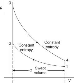
The basic Otto cycle is made up of four processes:

• Isentropic compression 1-2• Constant volume heat addition 2-3• Isentropic expansion 3-4• Constant volume heat rejection 4-1

The thermal efficiency of the Otto cycle:

`η =1−1/(cr^(γ−1)`_______________________(1)

where cr = compression ratio

the equation for isentropic compression and expansion process:

_____(2)

for solving above equation we create a function so that we easily call it during the main code

Assume:

• Bore diameter = 0.1 m
• Stroke length = 0.1 m
• Connecting rod=0.15 m
• compression ratio =12
• P1 =101325
• T1 = 500 k
• T3 = 2300 K

function [V]=engine_kinematics(b,stroke,c_rod,cr,start_crank,end_crank)

a= stroke/2;
r=c_rod/a;

theta= linspace(start_crank,end_crank,100)

t1=0.5*(cr-1);
t2=r+1-cosd(theta);
t3=(r^2-sind(theta).^2).^0.5;

%calculate volumn
v_swapt = (pi/4)*b*b*stroke;
v_c = v_swapt/(cr-1);

%isentropic equation
V= v_c*(1+t1*(t2-t3))


end

Explain:

• Here input of function is b,stroke,c_rod,cr,start_crank,end_crank
• create theta variable using linspace with length of 100 values.
• equation 2 divided into three part for calculation like t1,t2,t3.
• V gives values of volume as the piston moves from BDC to TDC or TDC to BDC depend on crank angle we define in function.

Error: error generates due to not define variable.solve by defining it.

Main MATLAB Code:

In this code, we call the function engine_kinematics in step 4 and 7;

%Generate PV Diagram of Otto cycle using MATLAB

close all
clear all
clc

%step 1:predefine state variables
p1=101325;
T1=500;
T3=2300;

%input values
b=0.1;
stroke=0.1;
c_rod=0.15;
cr=12;
gamma=1.4;

%step 2: calculate Volume
v_swapt = (pi/4)*b*b*stroke;
v_clearance = v_swapt/(cr-1);

v1= v_swapt + v_clearance;
v2 = v_clearance;

%step 3:calaculate value of p2 | p1v1^gamma =p2v2^gamma
p2 = p1*(cr)^gamma;

%step 4:genarate diffrent point between state point 1 to 2 compression process by using
%function
constant_c=p1*v1^gamma;
V_comprassion=engine_kinematics(b,stroke,c_rod,cr,0,180);
p_comprassion = constant_c./V_comprassion.^gamma;

%step 5:calculate state variable at point 2 | p1v1/T1 =p2v2/T2
T2 = T1*(p2/p1)*(v2/v1);

%step 6:calculate state variable at point 3 | Volume constant  
v3=v2;
% pressure at point 3 | p2v2/T2 = p3v3/T3
p3 = p2*(T3/T2);

%step 7:genarate diffrent point between state point 3 to 4 expansion process by using
%function
constant_c=p3*v3^gamma;
V_expansion = engine_kinematics(b,stroke,c_rod,cr,540,720);
p_expansion = constant_c./V_expansion.^gamma;

%step 8:calculate state variable at point 4 | constant volume
v4=v1;
p4 = p3/cr^gamma;

%step 9:calculate thermal efficiency
thermal_efficiency = 1-(1/cr^(gamma-1))

%step 10: Plot PV diagram
figure(1)
hold on
grid on
plot(V_comprassion,p_comprassion,'linewidth',1)
plot([v2 v3],[p2 p3],'linewidth',1)
plot(V_expansion,p_expansion,'linewidth',1)
plot([v4 v1],[p4 p1],'linewidth',1)
xlabel('Volome (m^3)')
ylabel('Pressure')
title('PV diagram of Otto Cycle')
legend('Isentropic compression','Constant volume heat addition','Isentropic expansion','Constant volume heat rejection')

PV diagram:

All values:

Thermal Efficiency:

Error: this error occurs due to I forget to define T3 at starting.

Conclusion: Here we get highly the accurate volume of a cylinder with variation in pressure so we get information at all point from PV diagram. Also by using this code, we calculate all values very quickly with less effort.