Curve fitting using MATLAB

Curve fit-

Curve fitting is the process of constructing a curve, or mathematical function, that has the best fit to a series of data points, possibly subject to constraints. Curve fitting can involve either interpolation, where an exact fit to the data is required, or smoothing, in which a "smooth" function is constructed that approximately fits the data.

A “good fit” might be a model

• That your data could reasonably have come from, given the assumptions of least-squares fitting
• In which the model coefficients can be estimated with little uncertainty
• That explains a high proportion of the variability in your data, and is able to predict new observations with high certainty

EVALUATING GOODNESS OF FIT-

1.Graphical(residual analysis ,confidence and prediction bounds)

2.Numerical (goodness of fit statistics)

A visual examination of the fitted curve displayed in Curve Fitting app should be your first step. Beyond that, the toolbox provides these methods to assess goodness of fit for both linear and nonlinear parametric fits:

• Goodness-of-Fit Statistics
• Residual Analysis
• Confidence and Prediction Bounds

1. Graphical-

(A)Plotting and Analysing Residuals-

The residuals from a fitted model are defined as the differences between the response data and the fit to the response data at each predictor value.

residual = data – fit

Mathematically, the residual for a specific predictor value is the difference between the response value y and the predicted response value ŷ.

Assuming the model you fit to the data is correct, the residuals approximate the random errors. Therefore, if the residuals appear to behave randomly, it suggests that the model fits the data well. However, if the residuals display a systematic pattern, it is a clear sign that the model fits the data poorly. Always bear in mind that many results of model fitting, such as confidence bounds, will be invalid should the model be grossly inappropriate for the data.

A graphical display of the residuals for a first degree polynomial fit is shown below. The top plot shows that the residuals are calculated as the vertical distance from the data point to the fitted curve. The bottom plot displays the residuals relative to the fit, which is the zero line.

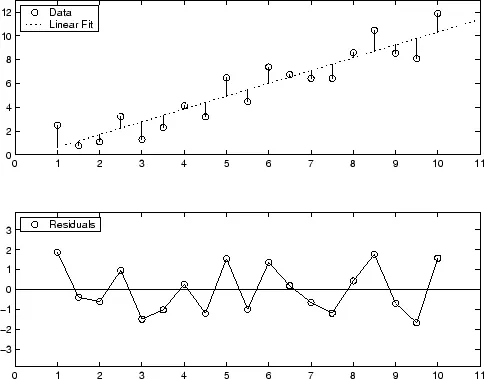
The residuals appear randomly scattered around zero indicating that the model describes the data well.

A graphical display of the residuals for a second-degree polynomial fit is shown below. The model includes only the quadratic term, and does not include a linear or constant term.

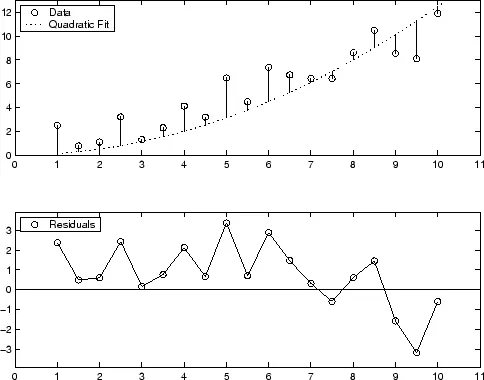
The residuals are systematically positive for much of the data range indicating that this model is a poor fit for the data.

(B)Confidence and prediction bounds-

Confidence and prediction bounds define the lower and upper values of the associated interval, and define the width of the interval. The width of the interval indicates how uncertain you are about the fitted coefficients, the predicted observation, or the predicted fit. For example, a very wide interval for the fitted coefficients can indicate that you should use more data when fitting before you can say anything very definite about the coefficients.

The bounds are defined with a level of certainty that you specify. The level of certainty is often 95%, but it can be any value such as 90%, 99%, 99.9%, and so on. For example, you might want to take a 5% chance of being incorrect about predicting a new observation. Therefore, you would calculate a 95% prediction interval. This interval indicates that you have a 95% chance that the new observation is actually contained within the lower and upper prediction bounds.

2. Numerical analysis-

Goodness-of-Fit Statistics-

After using graphical methods to evaluate the goodness of fit, you should examine the goodness-of-fit statistics. Curve Fitting Toolbox™ software supports these goodness-of-fit statistics for parametric models:

• The sum of squares due to error (SSE)
• R-square
• Adjusted R-square
• Root mean squared error (RMSE)

(a)Sum of Squares Due to Error-

This statistic measures the total deviation of the response values from the fit to the response values. It is also called the summed square of residuals and is usually labelled as SSE.

SSE=nXi=1wi(yi−ˆyi)2

A value closer to 0 indicates that the model has a smaller random error component, and that the fit will be more useful for prediction.

(b)R-Square-

This statistic measures how successful the fit is in explaining the variation of the data. Put another way, R-square is the square of the correlation between the response values and the predicted response values. It is also called the square of the multiple correlation coefficient and the coefficient of multiple determination.

R-square is defined as the ratio of the sum of squares of the regression (SSR) and the total sum of squares (SST). SSR is defined as

SSR=nXi=1wi(ˆyi−‾y)2

SST is also called the sum of squares about the mean, and is defined as

SST=nXi=1wi(yi−‾y)2

where SST = SSR + SSE. Given these definitions, R-square is expressed as

R-square=SSRSST=1−SSESST

R-square can take on any value between 0 and 1, with a value closer to 1 indicating that a greater proportion of variance is accounted for by the model. For example, an R-square value of 0.8234 means that the fit explains 82.34% of the total variation in the data about the average.

If you increase the number of fitted coefficients in your model, R-square will increase although the fit may not improve in a practical sense. To avoid this situation, you should use the degrees of freedom adjusted R-square statistic described below.

Note that it is possible to get a negative R-square for equations that do not contain a constant term. Because R-square is defined as the proportion of variance explained by the fit, if the fit is actually worse than just fitting a horizontal line then R-square is negative. In this case, R-square cannot be interpreted as the square of a correlation. Such situations indicate that a constant term should be added to the model.

(c)Degrees of Freedom Adjusted R-Square-

This statistic uses the R-square statistic defined above, and adjusts it based on the residual degrees of freedom. The residual degrees of freedom is defined as the number of response values n minus the number of fitted coefficients m estimated from the response values.

v = n – m

v indicates the number of independent pieces of information involving the n data points that are required to calculate the sum of squares. Note that if parameters are bounded and one or more of the estimates are at their bounds, then those estimates are regarded as fixed. The degrees of freedom is increased by the number of such parameters.

The adjusted R-square statistic is generally the best indicator of the fit quality when you compare two models that are nested — that is, a series of models each of which adds additional coefficients to the previous model.

adjusted R-square=1−SSE(n−1)SST(v)

The adjusted R-square statistic can take on any value less than or equal to 1, with a value closer to 1 indicating a better fit. Negative values can occur when the model contains terms that do not help to predict the response.

(d)Root Mean Squared Error

This statistic is also known as the fit standard error and the standard error of the regression. It is an estimate of the standard deviation of the random component in the data, and is defined as

RMSE=s=GMSE

where MSE is the mean square error or the residual mean square

MSE=SSEv

Just as with SSE, an MSE value closer to 0 indicates a fit that is more useful for prediction.

Now let us write a program to fit a curve for data of cp values at given temperatures.

Objective-

• Write code to fit a linear and cubic polynomial for the Cp data.
• Plot the linear and cubic fit curves along with the raw data points

here in this program we use two functions -

1.Polyfit - using this command we fit a curve of particluar degree we want and the coefficients of the polynomial

2.Polyval- using the command we can use the formula give one of the parameter as input and get the other parameter as output.

Program with explanation-

Now we start with taking the file data.txt which contains various values of cp for coressponding temperatures.

close all
clear all
clc
%data input
cp_data=load('data')

Now we read the data column wise and store them into temperature and cp arrays.

temperature=cp_data(:,1)
cp=cp_data(:,2)

Now using the polyfit and polyval commands we fit the data and caluclate the coressponding coefficients.

coefficients=polyfit(temperature,cp,1)
predicted_cp=polyval(coefficients,temperature)

Here we used polyfit command and give our temperature and cp values as input.since we want make a linear fit we gave the degree as one.

Later we use polyval command to predict the values of cp using the equation coefficients we obtained by polyfit and store it another array predicted_cp.

Now we need to plot the data of initial cp and temperature values and predicted cp and temperature values,we define the axis and turn on the legend to clearly differentiate between the two curves.

%plotting
figure(1)
plot(temperature,cp)
hold on
plot(temperature,predicted_cp)
xlabel('temperature[K]')
ylabel('specific heat[ KJ/K mol- K]')
legend('original data set','predicted set')

So similarly we also do the same thing to obtain a cubic fit,but we need to change the degree of the polynomial as 3,and plot the same graphs.

%for a cubic polynomial
coefficients2=polyfit(temperature,cp,3)
predicted_cp2=polyval(coefficients2,temperature)
figure(2)
plot(temperature,cp)
xlabel('temperature[K]')
ylabel('specific heat [KJ/K mol- K]')
hold on
plot(temperature,predicted_cp2)
legend('original data set','predicted set2').

Program-

close all
clear all
clc
%data input
cp_data=load('data')
temperature=cp_data(:,1)
cp=cp_data(:,2)
coefficients=polyfit(temperature,cp,1)
predicted_cp=polyval(coefficients,temperature)
%plotting
figure(1)
plot(temperature,cp)
hold on
plot(temperature,predicted_cp)
xlabel('temperature[K]')
ylabel('specific heat[ KJ/K mol- K]')
legend('original data set','predicted set')
%for a cubic polynomial
coefficients2=polyfit(temperature,cp,3)
predicted_cp2=polyval(coefficients2,temperature)
figure(2)
plot(temperature,cp)
xlabel('temperature[K]')
ylabel('specific heat [KJ/K mol- K]')
hold on
plot(temperature,predicted_cp2)
legend('original data set','predicted set2')

Output-

As we can see in the picture there is a difference in both the curve fit as the degree of the polynomial changes .But inorder to get all the properties `we use the matlab curve fit tool.

Using the curve fit tool we give the input values and get the curve fit for polynomial degree

1.

We can get the values of SSE,R-square,adjusted R-square,RMSE using this tool.

How to make the curve fit perfectly-

A curve is setb to be fitted perfectly if the predicted curve has less deviation from the original curve.

We can do it by scaling and centering option in the tool box.

Also as the degree of the polynomial is increased the curve gets fitted perfectly.

How to get the best fit-

Best fit is the fit where the deviation between the actual and predicted values is minimum.

we need to check for the goodness of fit statistics

• The sum of squares due to error (SSE)- The fit should have comparitively minimum value.
• R-square- The R-square value should be near to 1.
• Adjusted R-square
• Root mean squared error (RMSE).

By comparing all the quantities we can get the relatively best fit.

Improving cubic fit-

It can be done by scaling and centering it-

Program-

close all
clear all
clc
%data input
cp_data=load('data')
temperature=cp_data(:,1)
cp=cp_data(:,2)
a=1;
b=400;
for i=1:8%split the data
[coefficients,mu]=polyfit(temperature(a:b),cp(a:b),3)
predicted_cp(a:b)=polyval(coefficients,temperature(a:b),mu)
a=b+1;
b=b+400;
end
%plotting
figure(1)
plot(temperature,cp,'linewidth',2)
hold on
plot(temperature,predicted_cp,'linewidth',1)
xlabel('temperature[K]')
ylabel('specific heat[ KJ/K mol- K]')
legend('original data set','predicted set')

Output-

The plot is nearly scaled but as we zoom the picture we can still see a deviation between the curves which can be reduced by increasing the degree of the polynomial.

This is the zoomed picture-

Now if we use the curve tool and increase the degree of the polynomial we can observe that the curve fits well and also the goodness paramters are optimal

Here we used a five degree polynomial

Output tab-