CURVE FITTING FOR A LINEAR AND CUBIC POLYNOMIAL USING MATLAB

OBJECTIVE:

• To Write code to fit a linear and cubic polynomial for the Cp data.
• And to Plot the linear and cubic fit curves along with the raw data points.
• To Explain the parameters used to measure the fitness characteristics for both the curves.

THEORY:

CURVE FITTING

Curve fitting is the process of constructing a curve, or mathematical function, that has the best fit to a series of data points possibly subject to constraints. Curve fitting can involve either interpolation,where an exact fit to the data is required, or smoothing,in which a "smooth" function is constructed that approximately fits the data. A related topic is regression analysis, which focuses more on questions of statistical inference such as how much uncertainty is present in a curve that is fit to data observed with random errors.

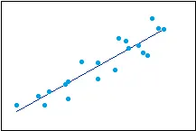
The first degree polynomial equation

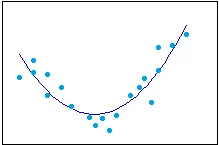
If the order of the equation is increased to a second degree polynomial, the following results:

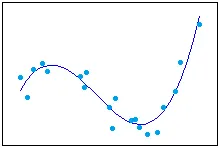
If the order of the equation is increased to a third degree polynomial, the following is obtained:

HOW TO CHOOSE THE BEST FIT

After using the graphical methods to evaluate the goodness of fit and the following method can be used for find out the best fit .

Sum of squares due to error(SSE)

R-Square

Adjusted R-Square

Root Mean Squared Error(RMSE).

Sum of squares due to error(SSE)

The total deviation of the response values from the fit to the response values. This statistic measures is also called as Sum of squares due to error(SSE).

R-Square

R-Square is the square of the correlation between the response values and the predicted response values. it is also called the square of the multiple correlation coefficient and the coefficient of multiple determination. This stattistic measures how successful the fit is in explaining the variation of data.

R-square is defined as the ratio of sum of the squares of regression(SSR) and the total sum of squares(SST). The Formula is defines below

SST is also called the sum of squares about the mean, where SST= SSR+SSE and is defined as

Adjusted R-Square

R² shows how well terms (data points) fit a curve or line. Adjusted R² also indicates how well terms fit a curve or line, but adjusts for the number of terms in a model. If you add more and more useless variables to a model, adjusted r-squared will decrease. If you add more useful variables, adjusted r-squared will increase.
Adjusted R² will always be less than or equal to R².

You only need R² when working with samples. In other words, R² isn’t necessary when you have data from an entire population.

The formula is:

where:

• N is the number of points in your data sample.
• K is the number of independent regressors, i.e. the number of variables in your model, excluding the constant.

Root Mean Squared Error(RMSE)

RMSD is a measure of accuracy, to compare forecasting errors of different models for a particular dataset and not between datasets, as it is scale-dependent. The root-mean-square deviation (RMSD) or root-mean-square error (RMSE) is a frequently used measure of the differences between values predicted by a model or an estimator and the values observed. The RMSD represents the square root of the second sample moment of the differences between predicted values and observed values or the quadratic mean of these differences.

INPUT PROGRAM:

CURVE FITTING TESTED USING FIRST ORDER

clear all
close all
clc

%preparing the data

cp_data = load('data');
temp = cp_data(:,1);
cp = cp_data(:,2);
%compare my curve fit with my original data
plot(temp,cp,'linewidth',1);
hold on

%curve fit
%cp = a*T^2+b*T+c

co_effs1 = polyfit(temp,cp,1);
predicted_cp = polyval(co_effs1,temp);

%compare my curve fit with my original data

plot(temp,predicted_cp,'linewidth',1)
xlabel('temperature [K]')
ylabel('specific heat [KJ/KMOL-K]')
legend('original plot','curve fit')

hold off

CURVE FITTING TESTED USING THIRD ORDER

clear all
close all
clc

%preparing the data

cp_data = load('data');
temp = cp_data(:,1);
cp = cp_data(:,2);
%compare my curve fit with my original data
plot(temp,cp,'linewidth',1);
hold on

%curve fit
%cp = a*T^2+b*T+c

co_effs3 = polyfit(temp,cp,3);
predicted_cp = polyval(co_effs3,temp);

%compare my curve fit with my original data

plot(temp,predicted_cp,'linewidth',1)
xlabel('temperature [K]')
ylabel('specific heat [KJ/KMOL-K]')
legend('original plot','curve fit')


hold off

CURVE FITTING TEST BY SPLITTING THE DATA INTO EQUAL PARTS

clear all
close all
clc

%preparing the data

cp_data = load('data');
temp = cp_data(:,1);
cp = cp_data(:,2);

%curve fit
%cp = a*T^2+b*T+c

co_effs1 = polyfit(temp,cp,1);
predicted_cp1 = polyval(co_effs1, temp);


co_effs3 = polyfit(temp,cp,3);
predicted_cp3 = polyval(co_effs3, temp);

% calculation for R square
% To split the curve using loop

sse = 0;
ssr = 0;
sum = 0;

for i = 1:length(cp)
    sum = sum+cp(i);
end 
mean = sum/length(cp);
for i = 1:length(cp)
    ssr = ssr+(predicted_cp1(i)-mean)^2;
    sse = sse+(cp(i)-(predicted_cp1(i)))^2;
end

sst = ssr+sse;
r_square = ssr/sst



sse = 0;
ssr = 0;
sum = 0;

for i = 1:length(cp)
    sum = sum+cp(i);
end 
mean = sum/length(cp);
for i = 1:length(cp)
    ssr = ssr+(predicted_cp3(i)-mean)^2;
    sse = sse+(cp(i)-(predicted_cp3(i)))^2;
end

sst = ssr+sse;
r_square = ssr/sst

%compare my curve fit with my original data
plot(temp,cp,'linewidth',1);
hold on
plot(temp, predicted_cp1,temp, predicted_cp3,'linewidth',1)
xlabel('temperature [K]')
ylabel('specific heat [KJ/KMOL-K]')
title('Splitwise Curve')
legend('originaldatafit','linear fit','cubic fit')
grid on

EXPLANATION FOR PROGRAM

• In this program the temperature and specific heat values are given by data files it contains of 3200 values. These values are used to plot the original datafit.
• Polynomial equation are equated to find the linear plot of graph to compare it with original datafit for error calculation.
• To obtain a better fit the 'splitwise' technique is been used, the number of splits is done by 10 equal divison from 1 to 3200 and the values of which is utilised for goodness of fit.
• For each split of data ,polyfit creates a new set of co-efficients which are used to polyval to output new values of spcific heat .
• New values of specific heat are calculated by the polyval is ploted in the graph against the temperature.
• To measure the goodness fit ,the r square statistical method is executed.
• R-square method is been done to understand the closeness to actual data.
• Output of the R-square is will be upto 0.99 to 1 that are refer as the best fit curve.

OUTPUT:

ERRORS FACED DURING THE PROGRAM:

In this error the co_eff are not defined properly and it doesn't takes the values of coefficent. The error is identified and rectified.

CONCLUSION:

• Curve fitting is used to analyse the 'noisy data' that has no given physical relation
• R-square value are calculated and testing of curvefit is done.
• So the curvefit is performed using MATLAB and it is found that lesser the degree of the polynomial higher the goodness of the curvefit.