Air Standard Cycle - Otto Cycle P-V Diagram & Efficiency Analysis

AIM:

To recreate the Otto Cycle using MATLAB and to analyse the thermal efficiency of the same.

OBJECTIVES:

- To code the Otto Cycle on MATLAB.

- To produce graphs of the required P-V diagram obtained in regards to the inputs conisdered.

- To obtain the thermal efficiency of the cycle under study.

THEORY:

- The Otto cycle is the main air standard cycle governing the operation of a gasoline spark ignition engine. It depicts the steps involved through which these heat engines convert gasoline into kinetic energy (motion). This process involves changing chemical energy into thermal energy before finally allowing for the vehicle to be set into motion.

- When considering the ideal Otto cycle, 4 main processes come into picture:

i) Isentropic Compression (1->2): The first step involves the piston moving upwards in order to compress the fuel-air mixture that is made to enter the combustion chamber during the intake phase (Green Line in the diagram below indicates the intake phase, that occurs at constant pressure, where the piston is initially located at the bottom before allowing for an increase in volume through the intake of the required fuel-air mixture). Here, the above mixture sees an increase in its temperature and pressure. However, the term 'Adiabatic' is used to define this step as no heat transfer is experienced. The fuel is made to be ignited at this stage.

ii) Constant Volume Heat Addition (2->3): Combustion occurs here through the use of the spark plug, causing a drastic increase in pressure. An increase in thermal energy occurs as well, but at a constant volume, therefore the word 'Isochoric Process' is used to desrcibe this stage of the cycle.

iii) Isentropic Expansion (3->4): At this stage, due to the thermal energy's effect, the piston moves down due to the work output seen from the previous stage, therefore causing an increase in the volume contained within the combustion chamber. Named the 'power stroke' of the cycle, this stage mainly results in the thermal energy's conversion into the motion of the vehicle. This process is an Adiabatic process as well.

iv) Constant Volume Heat Rejection (4->1,Blue Line): This is the final exhaust stage of the cycle where all residual heat is rejected from the engine. Due to this, as gas molecules lose their kinetic energy, a decrease in pressure is noticed. This is once again an Iscochoric process.

Once this cycle is completed, the engine proceeds to repeat the same to constantly provide power to allow for the vehicle's motion.

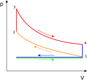
FIGURE: P-V Diagram of Ideal Otto Cycle

MATLAB PROGRAM:

A number of assumptions were taken initially in terms of engine geometric parameters as well as certain engine input parameters. This is necessary to do so as we require a certain amount of information in order to conduct the required analysis.

i) Engine Kinematics Function

function [V] = Ottokinematics(bore,stroke,conrod,cr,startcrank,endcrank)
a = stroke/2;
r = conrod/a;

v_sweptvol = (pi/4) * bore^2 * stroke;
v_clearence = v_sweptvol/(cr-1);
theta = linspace(startcrank,endcrank,100);

term1 = 0.5*(cr-1);
term2 = r + (1 - cosd(theta));
term3 = (r^2 - sind(theta).^2).^0.5;

V = (1+term1*(term2-term3)).*v_clearence;
end

ii) Main Program

clc
clear all
close all

%Defining Inputs


%Known State Variables
p1 = 101325; %Pressure @ Stage 1 (Pascals)
t1 = 300; %Temperture @ Stage 1 (kelvin)
t3 = 2300; %Temperature @ Stage 3
gamma = 1.4; %Specific Heat Ratio

%Engine Geometric Parameters
bore = 0.1; %Bore Diameter (m)
stroke = 0.1; %Stroke Length (m)
conrod = 0.16; %Connecting Rod Length (m)
cr = 12; %Compression Ratio

SVol = (pi/4) * bore^2*stroke; %Swept Volume
CVol = SVol / (cr-1); %Clearence Volume

v1 = SVol + CVol ;
v2 = CVol;

%State 2 Variable
%Using Equation: p2(v2^gamma)=p1(v1^gamma), we find pressure.
%We know that v1^gamma/v2^gamma = Compression Ratio, cr
p2  = p1 * cr^gamma;

%To calculate temperature @ State 2
%Using Equation: p1v1/t1=p2v2/t2
t2 = (p2*v2*t1) / (p1*v1);

%For Isentropic Equation: Constant c=pv^gamma
c = p1*v1^gamma;

%Calculating Isentropic Compression
v_compress = Ottokinematics(bore,stroke,conrod,cr,0,180);
p_compress = c./v_compress .^gamma;

%State 3 Variables
v3=v2
p3=(p2*t3)/t2
c = p3*v3^gamma;

%Calculating Isentropic Expansion
v_expan = Ottokinematics(bore,stroke,conrod,cr,180,360);
p_expan = c./v_expan .^ gamma;

%State 4 Variables
v4 = v1
p4 = p3 * (v3/v4)^gamma; %Using p3v3^gamma=p4v4^gamma

%Thermal Efficiency
n = (1 - 1/(cr^(gamma-1)))*100 %Returns efficiency in percentage

%Plotting
figure (1)
hold on
plot ([v2 v3],[p2 p3])
plot ([v4 v1],[p4 p1])
plot (v_compress,p_compress)
plot (v_expan,p_expan)
plot (v1,p1,'*','color','r')
plot (v2,p2,'*','color','r')
plot (v3,p3,'*','color','r')
plot (v4,p4,'*','color','r')
xlabel('Volume')
ylabel('Pressure')

FIGURE: P-V Diagram Obtained (Using Assumed Parameters)

CONCLUSION:

Once the coding for the MATLAB was executed correctly, the P-V diagram was then accurately attained before realising the thermal efficincy obtained from the same to be: 62.99%.

REFERENCES:

- Otto Cycle: https://energyeducation.ca/encyclopedia/Otto_cycle

- Otto Cycle P-V Diagram: https://energyeducation.ca/wiki/images/thumb/8/89/P-V_Otto_cycle.png/600px-P-V_Otto_cycle.png