2D Cavitation simulation

Introduction: In the engine, fuel passes from the complex path to reach the combustion chamber during this path due to sudden changes in the area the pressure of fuel increases or decreases.

In this project, we will be focusing on how fuel flow induces cavitation when it enters the combustion chamber through a Winkl Hoffer nozzle.

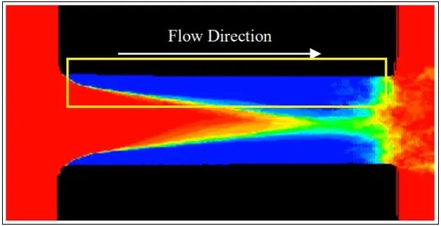
As we can see in the above image when fuel passes from the fuel chamber into the throat of the nozzle there is an abrupt change in the area and because of this, there is an abrupt change in flow radius this causes a huge low-pressure region or area of separation as we can see in the above image.

Here the cavitation forms when the static pressure of the fluid drops below the vapor pressure of the fluid in the low-pressure region and this drop in static pressure will the vapourize the fluid flow into the gaseous phase instantaneously and this will affect the injector properties in terms of delivering the required fuel flow rate & this subsequently affects the combustion performance & emissions performance & that’s why in automotive applications studying cavitation is extremely important.

Objective: To Study cavitation in Winkl Hoffer Nozzle using Converge CFD

Theory: In our case, we have both liquid & gas phase so, in order to run this type of simulation, we will use the Volume of fluid methodology the volume of fluid is basically the subset of the Multiphase flow simulation

In Converge CFD, the transition from the liquid phase to the gas phase is described by the following rate law:

`frac{dx}{dt}=frac{overlinex-x}{theta}`

`frac{dx}{dt}=`tells the rate at which liquid gets converted into vapor

`theta`=time scale

`theta=thetaunderset(0)()xxalpha^(-0.54)xxpsi^-1.76`

where,

`thetaunderset(0)` is a coefficient set to 3.84e-7

`alpha`=total void fraction

`psi` =total dimensional pressure ratio =`frac{Punderset(sat)()-P}{Punderset(crit)()-Punderset(sat)()`

This time scale is calculated from below empirical relation which is been created from experiments:

Geometry:

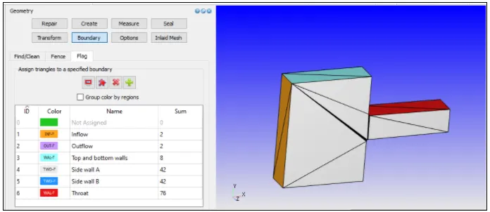
The pre-modeled geometry was imported into Converge and the geometry was inspected for surface error or other errors. After fixing all the errors & the boundaries were flagged & case was set up.

Case setup:

Simulation Type:

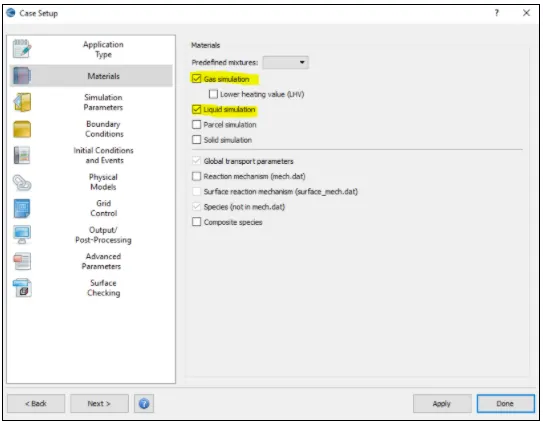
From the above image, the reason behind enabling both gas & liquid simulation is because we are simulating Multiphasse simulation.

Materials: For materials we have enabled 2 properties

• Liquid tetradecane(IC14H30)
• Gas tetradecane(C14H30)

Initially, in the domain, there will be only liquid tetradecane & when the cavitation occurs the liquid tetradecane(IC14H30) will be converted into gas tetradecane(C14H30).

Solver: Transient solver

Simulation mode: Full hydrodynamic

Region & Initialization:

• In this step, we have created a region of the fluid and initialize the pressure as 106Pa & also the species value as IC14H30= 0.99998 & N2=2e-05

Boundary Conditions:

All the boundary conditions are defined at temperature=300K.

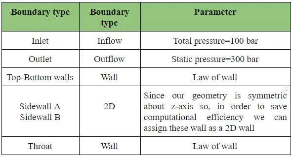
From the above table, we can see that there is a huge pressure drop which is around 70 bar and this pressure will drive the velocity very high and this form simulation as velocity based CFL number or convection based CFL number so, in convection based CFL number the maximum convection CFL limit should not be more than 0.5 which we can in the below image:

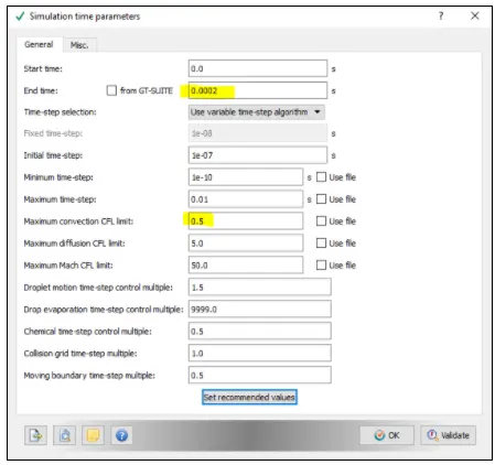
From the above image we can see that our Simulation time parameter is:

• Start time:0 sec
• End time:2 milliseconds

The reason behind choosing 2 milliseconds as an end time is because typically injection takes place for this much amount of time.

Physical Model

• Turbulence model:k_e-epsilon
• VOF model: Basic VOF
  • The basic idea here is that the VOF will solve one transport equation for liquid phase & one transport equation for gas-phase & interface between liquid and gas phase will get calculated automatically.

Grid Control:

• Element size:dx = 4e-5m, dy = 4e-5m & dz = 4e-5m

AMR:

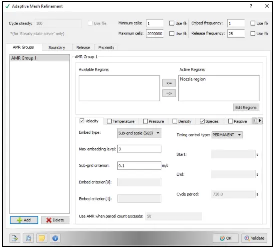
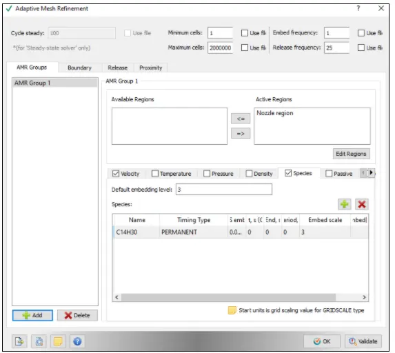
It’s essential to capture the data accurately were the cavitation occurs, so for this, we need more refine mesh or local mesh in that area while keeping the mesh size in the other area as same as the base grid size so, in order to do this we are using Adaptive mesh refinement technique.

In converge, adaptive mesh refinement gives a variety of based techniques in our case we will use velocity-based sub-grid-criterion & species-based sub-grid-criterion with two-layer. Converge will monitors the curvature of velocity & species property provided in the AMR and refines the mesh when the property of velocity & species curvature between the consecutive grid is more than the defined SGS value.

AMR use the below formula to determine the refine grid size

Refined Mesh=`frac{Base grid}{2^(Max embedded Level)}`

Velocity-based AMR

Species-based AMR

Fixed Embedding

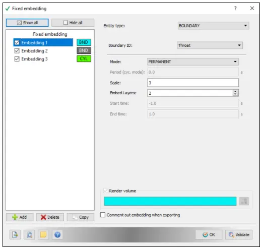
Fixed embedding is a method that is used to refine the mesh in a particular area. In our case, we are more concerned about the area near the throat & Top-bottom walls so, for this, we have used a fixed embedding method which as follows

Fixed embedding use the below formula to determine the refine grid size

Refined Mesh=`frac{Base grid}{2^(SCALE)}`

• 

Output Files:

• The time interval for writing 3D output data files: 5e-05 sec
• The time interval for writing text output:1e-10 sec
• The time interval for writing restarting output:1e-05 cycles
• The maximum number of restart file saved:5

Post-Processing:

Mesh:

Total cell count plot:

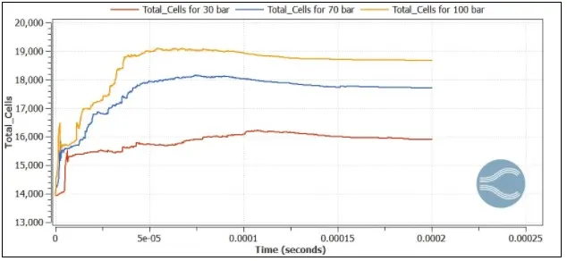
From the above plot, we can see that the total cell count changes which is because of AMR which we have used

Mass flow rate:

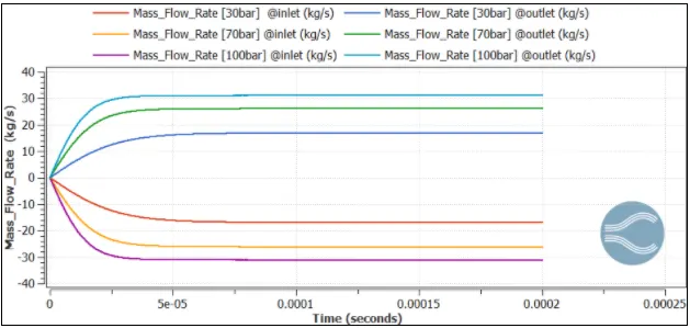
From the above plot, as we can see that the mass flow rate at the inlet is equal to the mass flow rate at the outlet which confirms that mass is conserved.

Also, we can see that there is a fluctuation in the mass flow rate which is because of cavitation.

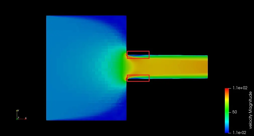
Velocity contour:

When the Pressure difference is 30 bar

When the Pressure difference is 70 bar

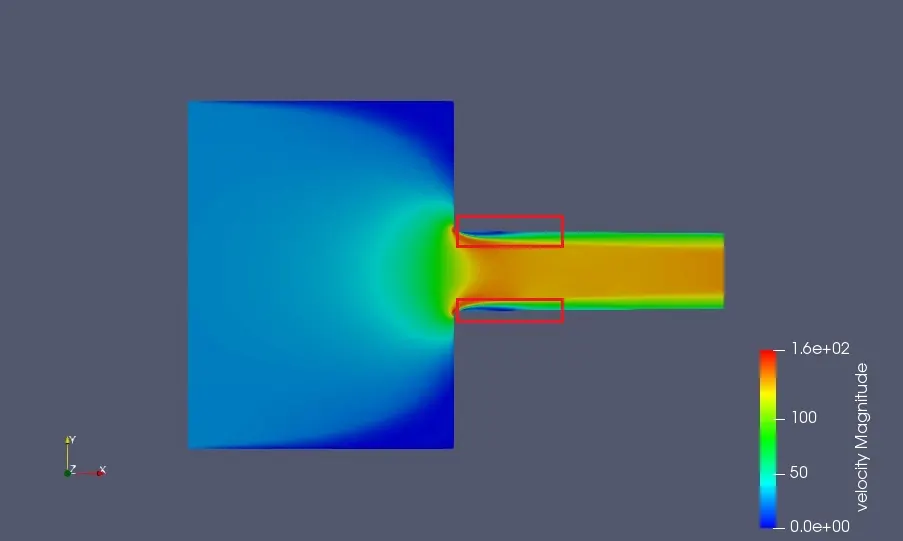
When the Pressure difference is 100 bar

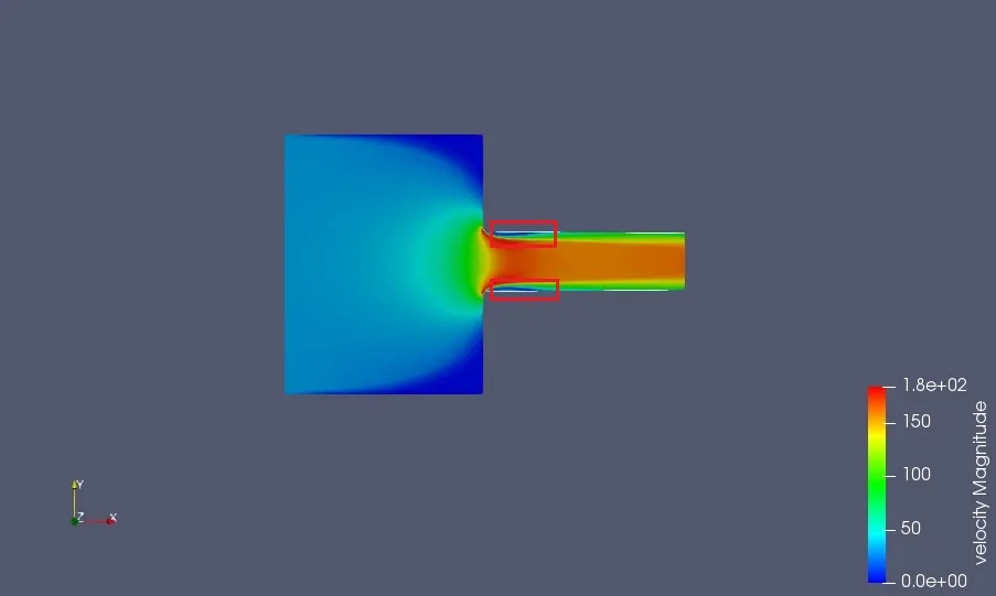
From the above velocity contours, we can see that at the throat due to sudden contraction in the area the velocity reaches the maximum also when we compare the above velocity contours amongst each other we can see that as pressure difference increases the velocity increases at the throat.

At the throat, due to sudden contraction in the area, a layer of fuel that is flowing along the wall gets separated and creates a flow separation.

Tn the flow separation region, when the static pressure of the fuel falls below the vapor pressure of the fuel the cavitation occurs.

Mass flow rate contour & its plot at the outlet:

When the Pressure difference is 30 bar

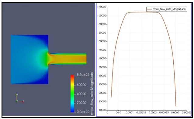
When the Pressure difference is 70 bar

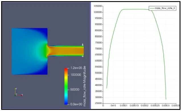
When the Pressure difference is 100 bar

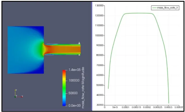
From the above contour, we can see that at the outlet the mass flow rate is not uniform, and this fluctuation in mass flow rate creates an improper injection of fuel spray which creates an improper air-fuel mixture and this improper air-fuel mixture will increase the emissions.

Velocity animation

Conclusion:

Successfully did a 2D cavitation simulation by taking Winkl-Hoffer Nozzle as a model also studied how cavitation occurs in injectors and the effect of cavitation in system performance.