Under Relaxation Factors: How to Get the Most Out of Your CFD Simulations

Under Relaxation Factors: How to Get the Most Out of Your CFD Simulations

CFD Simulations are carried out based on Navier Stoke equations. I.e., continuity equation, momentum equation, and energy equations.

After discretization, the guess value is given as input to all cells created in the domain. These guess values are interpolated over different iterations to obtain convergence. But to obtain the convergence at optimal conditions, a particular term called the under-relaxation factor is introduced. Under-relaxation factors are provided for different variables in different types of simulations.

Relaxation factors play a vital role in determining the rate of convergence for CFD simulation. For instance, for a stable solution with respect to combustion modeling, lower relaxation factors are required. When the relaxation factor is less than one, it is said to be under-relaxed, and it is called over-relaxed when the relaxation factor is more than one. The relaxation factor is always a constant, and it is multiplied by the algebraic equations to alter the path of the iteration. Changing the under-relaxation factors changes the convergence behavior of the CFD simulations. This is a technique used for improving the stability of a calculation, especially in solving steady-state analysis, where the first iterations are critical.

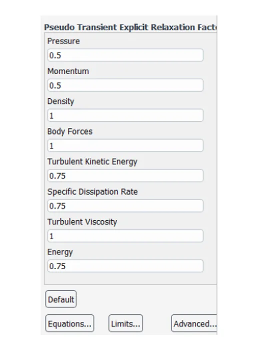
Most of the problems in fluid mechanics are solved using the Gauss-Jordan technique or Gauss-Seidel iterative method. Relaxation factors are used to get the results When the under-relaxed values are applied to the successive iterations of the above-mentioned methods, the convergence rate of the solution increases. The real challenge is to determine the best relaxation factor, which is only possible through a trial and error method. The optimum value of the relaxation factor is purely mesh dependent and is specific to a particular problem. However, it will be advantageous if we can select a relaxation parameter that minimizes the number of iterations required while conserving the stability of the solution as well.

Under-Relaxation

The method of under-relaxation is basically limiting the amount by which variable changes from the previous iteration to the next one. Due to the nonlinearity in the equations, it is important to control the change of the variable.

Because of the non-linearities of the equations being solved, it is necessary to control the change of variable φ. This is achieved by under-relaxation as follows:

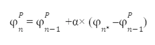
Where α is the factor that defines the relaxation such that:

• α < 1 , stability is more but the convergence rate is reduced, it means under-relaxation.
• α = 1 means no relaxation at all. The convergence rate or stability is unaffected by the relaxation factor
• α > 1 means over-relaxation. It can accelerate the convergence rate but also reduces the stability.

And:

• n refers to the new, used value of φP ;
• n−1 refers to the previous value of φP;
• n∗ refers to the new, predicted value of φP.

This means that the new value of the variable φ depends upon the old value, the computed change of φ, and α.

Pressure correction factor

In the staggered grid, the velocity components are calculated for the points that lie on the faces of the control volumes. The x-direction velocity u is calculated at the faces that are normal to the x-direction. The calculation of the diffusion coefficient and the mass flow rate at the faces of the u control volume would require an appropriate interpolation. The resulting discretization equation can be written as

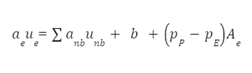
Here the number of neighbor terms will depend on the dimensionality of the problem. For the two-dimensional situation four u neighbors are shown outside the control volume; for a three-dimensional case, six neighbor u's would be included. The neighbor coefficients anb account for the combined convection-diffusion influence at the control-volume faces.The term (pP-pE)Ae is the pressure force acting on the u control volume, A, being the area on which the pressure difference acts.

The momentum equations can be solved only when the pressure field is given or is somehow estimated. Unless the correct pressure field is employed, the resulting velocity field will not satisfy the continuity equation. Such an imperfect velocity field based on a guessed pressure field p* will be denoted by u*, v*, w*. This "starred" velocity field will result from the solution of the following discretization equations:

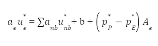
To improve the guessed pressure p* such that the resulting starred velocity field will progressively get closer to satisfying the continuity equation, a correct pressure p is proposed as

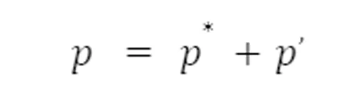
where p' will be called the pressure correction. We need to know how the velocity components respond to this change in pressure. The corresponding velocity corrections u', v', w' can be introduced as

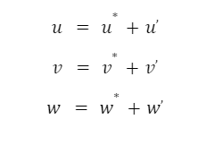
If we subtract the above Equations, we get

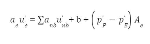
Where

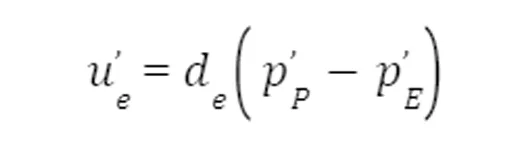
The above equation is stated as a velocity-correction formula

The pressure-correction equation derived is also prone to divergence unless some under-relaxation is used. Many different under-relaxation practices can be devised.

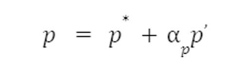
We under-relax u*, v*, w* while solving the momentum equations with a relaxation factor mentioned in the above article. p is known as pressure correction under the relaxation factor. p is usually given a value of 0.8 and =0.5 in the SIMPLE algorithm.