How Ode45 Takes the Pain Out of Solving Higher Order Derivatives

How Ode45 Takes the Pain Out of Solving Higher Order Derivatives

Introduction to ODE45

ODE45 is a standard MATLAB solver used to solve first-order ordinary differential equations. The function ODE45 implements a Runge-Kutta method with a variable time step for its computation.

ODE45 can compute an ODE of the form,

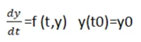
where t is the independent variable, y is a vector of dependent variables to be found, and f (t, y) is a function of t and y. The function f (t, y) is set, and the initial condition which is the value of the function at t=0s. i.e. y = y0 at time t0 are given.

Syntax for ODE45

The function ode45 takes 3 inputs. The 3 inputs are the function to be integrated, the time span and the initial conditions.

The time span would be the integration limits. This can be provided as a vector of 2 values, the initial and final time or with a spacing using the linspace function. The solver will choose a step size that is most suitable for the solution to obtain the solution in the most optimal time as possible. The initial condition would be the value of the function at t=0s.

The function can be provided in the form of an anonymous function,

[t,results] = ode45(@(x) x^2, tspan,y0)

Here, we are saying that we don’t know the value of x and that x is an input to the anonymous function that we have defined here. This is equivalent to defining a function that takes the input of x and gives the output of x^2.

The function can also be defined as a separate function. This function must take at least 2 inputs, which should be t and y, apart from other arguments, where t would be the current time and y would be the value of the function at the previous time step.

Assuming we have a function ode, the function must be defined as,

function [output] = ode(t,y,args)

where args refer to any other arguments that the function may take.

This function must then be input to ode45 as

[t,results] = ode45(@(t,y) ode(t,y,args), tspan, y0)

This is necessary to tell the function which arguments of the function are to be found by the solver.

Ode45 for higher-order derivatives

How Ode45 takes the initial conditions.

Let us take an example of 3rd-order ODE.

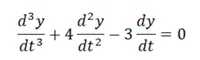
For 3rd order derivative we have 3 initial conditions which can be initialized in an array as follows.

At time t=0 , [I.C- 1, 1.C- 2, I.C-3] (I.C=Initial condition)

Lets us consider the example given below.

Initial conditions given at t =0 for `y` ,`dy/dt` and `(d^2y)/(dt^2)`

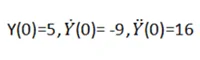
We can initialize the initial condition as an array as follows.

[5 -9 16]

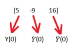
How ODE45 communicates

For a higher order derivative we need to reduce it into various first order differential equation. For example a 3rd order ODE must be split into three 1st order ODE.

Basically, you could have an ODE of any arbitrary order. What is important is that you reduce them to multiple 1st order ode's. Ode45 stores the results as state vectors, so if Y is the solution array, it will store the values as follows,

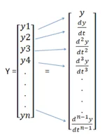
The above higher order derivatives can be represented as multiple 1st order derivatives in terms of state vectors i.e.

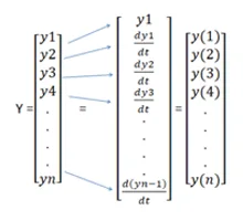
The results for Y will be stored as state vectors as shown above. y1,y2,y3,y4…yn are called the state variables.

So any higher order differential equation can be represented as a state vector.

So in our given example,

We can represent the above equation in terms of state vector. So this can done as follows:

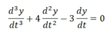
How to write an external function for the above example

Assuming we have a function ode the above example, the function can be defined as,

function [Ydot] = odefun(t,y)

Ydot=zeros(3,1)

Ydot(1)=y(2)

Ydot(2)=y(3)

Ydot(3)=3*y(2)-4*y(3)

end

Finally, the function can be called in main program as:

Ode45(‘Odefun’, tspan, I.C)