Breaking Ice with Air Cushion Vehicle - Find minimum pressure with Newton - Raphson Method
Aim:
To write a python script to solve for the minimum value of pressure using the Newton Raphson Method.
Objective:
1. To use the Newton Raphson Method to find out the value of pressure for h = 0.6 ft.
2. To find the optimal relaxation factor for this problem with the help of a suitable plot.
3. Tabulate the results of p for h = [0.6,1.2,1.8,2.4,3,3.6,4.2] assuming a suitable relaxation factor.
Theory:
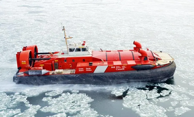
The ice sheet can be broken into small slabs with a heavy air-cushion vehicle (ACV) traveling on the float ice sheet at the critical speed. Ice-breaking with ACV is a new ice-breaking method in In-land River which has an important application in the prevention of ice jam flood in the Yellow River. In this paper, the icebreaking process of ACV is numerically simulated under shallow water and thick ice sheet condition. According to the simulating results, ACV traveling at the critical speed always chases after and pushes the wave crest ahead of ACV. Thus, the amplitude of the wave around ACV gradually increases due to the continual push of ACV. Ice sheet cracks when the stress and strain in the ice sheet accumulated to the critical value of failure. The critical speed of ACV should consist of the velocity of the surface wave around ACV. Under the thick ice sheet and shallow water environment in this paper, the critical speed of ACV is estimated as the velocity of a surface wave with a wavelength about the triple length of the ACV hull.
New Raphson Method:
The Newton-Raphson method (also known as Newton's method) is a way to quickly find a good approximation for the root of a real-valued function f(x)=0">f(x)=0f(x)=0. It uses the idea that a continuous and differentiable function can be approximated by a straight line tangent to it.
How it works...
Suppose you need to find the root of a continuous, differentiable function f(x)f(x)">f(x)f(x)f(x)f(x), and you know the root you are looking for is near the point x=x0">x=x0x=x0.
Then Newton's method tells us that a better approximation for the root is x1=x0-f(x0)f′(x0)">x1=x0−f(x0)f'(x0)x1=x0-f(x0)f′(x0).
This process may be repeated as many times as necessary to get the desired accuracy. In general, for any x-">x−x-value xn">xnxn,
the next value is given by xn+1=xn-f(xn)f′(xn)">xn+1=xn−f(xn)f'(xn)xn+1=xn-f(xn)f′(xn)
Note: the term "near" is used loosely because it does not need a precise definition in this context. However, x0">x0x0 should be closer to the root you need than to any other root (if the function has multiple roots).
Geometric Representation:
Here is a picture to demonstrate what Newton's method actually does:
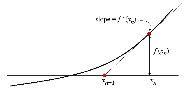
We draw a tangent line to the graph of f(x)">f(x)f(x) at the point x=xn">x=xnx=xn. This line has slope f′(xn)">f'(xn)f′(xn) and goes through the point (xn,f(xn))">(xn,f(xn))(xn,f(xn)). Therefore it has the equation y=f′(xn)(x-xn)+f(xn)">y=f'(xn)(x−xn)+f(xn)y=f′(xn)(x-xn)+f(xn). Now, we find the root of this tangent line by setting y=0andx=xn+1">y=0andx=xn+1y=0andx=xn+1 for our new approximation. Solving this equation gives us our new approximation, which is xn+1=xn-f(xn)f′(xn)">xn+1=xn−f(xn)f'(xn)xn+1=xn-f(xn)f′(xn).
Governing Equation:
f(x)=p3(1-β2)+(0.4hβ2-σh2r2)p2+σ2h43r4p-(σh23r2)3">f(x)=p3(1−β2)+(0.4hβ2−σh2r2)p2+σ2h43r4p−(σh23r2)3f(x)=p3(1-β2)+(0.4hβ2-σh2r2)p2+σ2h43r4p-(σh23r2)3,
On differentiating the f(x)">f(x)f(x) we get,
f′(x)=3p2(1-β2)+2p(0.4hβ2-σh2r2)+σ2h43r4">f'(x)=3p2(1−β2)+2p(0.4hβ2−σh2r2)+σ2h43r4f′(x)=3p2(1-β2)+2p(0.4hβ2-σh2r2)+σ2h43r4
Where, p">pp denotes the cushion pressure,
β">ββ related to the width of the ice-wedge,
h">hh is the thickness of the ice field,
σ">σσ is the tensile strength of the ice,
r">rr is the size of the air cushion.
Solution Procedure:
- Initially, all the required modules are imported viz., Math, NumPy, Matplotlib, and required inputs are given.
- Consider an array of h">hh and assume the value of α">αα as stated in the question.
- After that two different functions such as f(x)andf′(x)">f(x)andf'(x)f(x)andf′(x) is defined from the given formula, and an empty array to stored pressure and no. of iterations.
- To calculate minimum pressure for different values of ice thickness a for loop is executed taking an initial guess value of pressure and tolerance and ct = 1 which will increment after every iteration.
- And while loop is initiated to check whether all the absolute inputs in the formula is greater than tolerance provided.
- The new value of pressure is calculated using the Newton Raphson Method.
- All the new values are stored using append and we could plot the graph for pressure versus ice thickness using the calculated data set.
- For calculating optimal relaxation factor (α)">(α)(α) for given ice thickness and now the changes I made is the use of NumPy i.e., an array of α">αα range from 0.1 to 1.9 and the no. of points between them is 80 and value of h">hh_1 is taken as 1.2.
- and everything is the same for 'for loop' and 'while loop' mention in above one of the points.
- And the graph is plotted between no. of iterations and relaxation factor.
Python Code for this program:
"""
A program to calculate the minimum value of pressure for the given thickness of the icefield
"""
import math
import numpy as np
import matplotlib.pyplot as plt

# Inputs:...
# Beta is related to the width of ice wedge
beta = 0.5
# "r" is the size of the air cushion (feet)
r = 40
# "sigma" is the tensile strength of the ice (pounds per square inch (psi))
sigma = 150
# 1 foot = 12 inches | 1 square feet = (12*12) = 144 square inches
sigma = 21600
# "h" is the thickness of ice field
h = [0.6,1.2,1.8,2.4,3.0,3.6,4.2]
# Relaxation  factor (let say...)
alpha = 1.1

def f(p,h,r,beta,sigma):
	term1  = ((p**3)*(1-(beta**2)))
	term2a = (0.4*h*(beta**2))
	term2b = ((sigma*(h**2))/(r**2))
	term3  = (((sigma**2)*(h**4))/(3*(r**4)))
	term4  = ((sigma*(h**2))/(3*(r**2)))
	term01 = term1 + ((term2a - term2b)*(p**2)) + (term3*p) - (term4**3)
	return term01

def fprime(p,h,r,beta,sigma):
	term5  = (3*(p**2)*(1-(beta**2)))
	term6a = (0.4*h*(beta**2))
	term6b = ((sigma*(h**2))/(r**2))
	term7  = (((sigma**2)*(h**4))/(r**4))
	term02 = (term5) + (2*(term6a -term6b)*p) + (term7/3)
	return term02

# Empty array to store pressure after each iterations
pressure = []   # pound per square feet
pressure_0 = [] # pound per square inch (psi)

# empty array to store the no. of iterations
num_1 = []

for i in h:
	# Assuming initial pressure value
	p_guess = 101
	# Tolerance
	tolerance = 1e-6

	ct =1
	while(abs(f(p_guess,i,r,beta,sigma)) > tolerance):
		p_guess = p_guess - alpha*(f(p_guess,i,r,beta,sigma)/fprime(p_guess,i,r,beta,sigma))
		ct += 1
	pressure.append(p_guess)
	pressure_0.append(p_guess/144)
	num_1.append(ct)

print('Thickness of the Ice wedge :n',h)
print('Cushion pressure (pound per square feet :n', pressure)
print('Cushion pressure (psi) :n',pressure_0)
print('No. of iterations :n', num_1)

# Plotting of graph
plt.figure(1)
plt.plot(h, pressure, marker = 'o', color = 'maroon', markerfacecolor = 'green', markersize = 6)
plt.title('Cushion pressure Vs Ice field thickness', color = 'blue')
plt.xlabel('Thickness of Ice field (feet)', color = 'green')
plt.ylabel('Cushion pressure (pound per square feet)', color = 'green')
plt.grid()
plt.show()

# Plotting of graph
plt.figure(2)
plt.plot(h, pressure_0, marker = '*', color = 'maroon', markerfacecolor = 'yellow', markersize = 8)
plt.title('Cushion pressure Vs Ice field thickness', color = 'blue')
plt.xlabel('Thickness of Ice field (feet)', color = 'green')
plt.ylabel('Cushion pressure (psi)', color = 'green')
plt.grid()
plt.show()

"""
 Question (2)
Program to calculate optimal relaxation factor for a given thickness of Ice field
"""

# let us take h_1 the thickness of the ice field
h_1 = 1.2
# By considering both the underrelaxing and overrelaxing values in the Relaxation factor array
alpha_a = np.linspace(0.1,1.9,80)

num = []

for j in alpha_a:
	# Assuming pressure value
	p_guess = 101
	# Tolerance
	tolerance = 1e-6

	ct = 1
	while (abs(f(p_guess,h_1,r,beta,sigma)) > tolerance):
		p_guess = p_guess - (j*f(p_guess,h_1,r,beta,sigma))/fprime(p_guess,h_1,r,beta,sigma)
		ct +=1
	num.append(ct)
	#print(num)
	print(j)

# Plotting the graph
plt.figure(3)
plt.plot(alpha_a,num,marker = '.',color = 'black',markerfacecolor = 'red',markersize = 6)
plt.title('No. of Iterations Vs Relaxation factor', color = 'blue')
plt.xlabel('Relaxation factor(alpha)', color = 'green')
plt.ylabel('No. of Iterations', color = 'green')
plt.grid()
plt.show()Result:
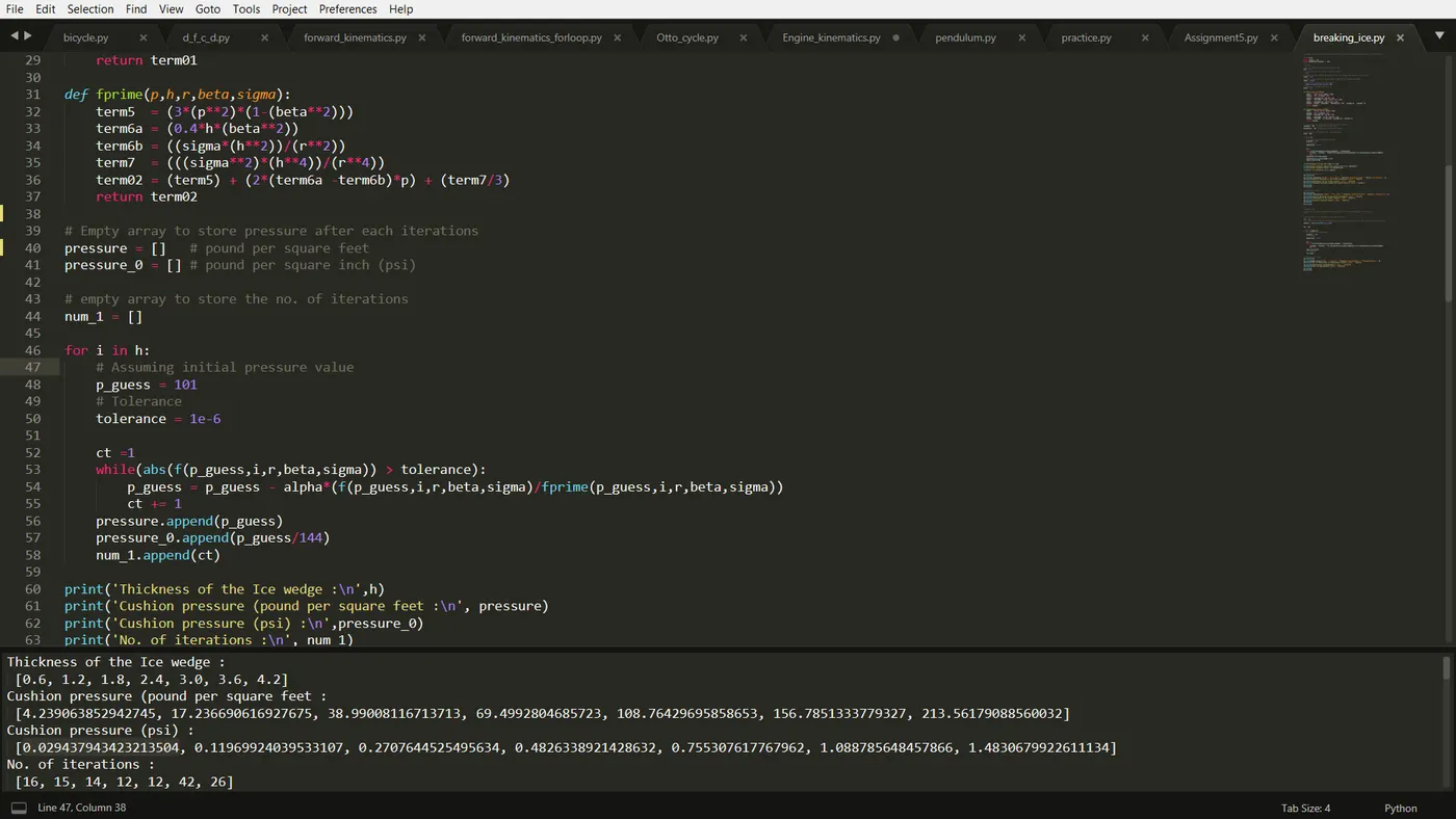
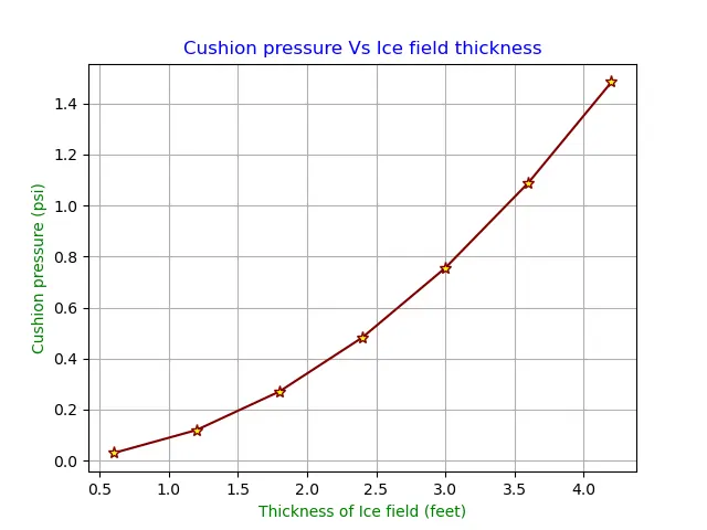
The value of pressure in both the units gives 4.239063852942745 pounds per square feet and 0.029437943423213504 (psi) respectively for 0.6 thickness of the ice field.
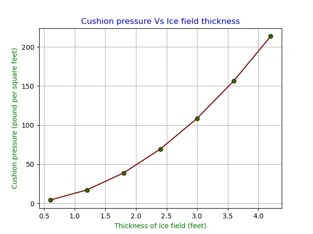
The graph shows the variation of pressure with the thickness of the ice field.....
The graph for optimal relaxation factor for the given ice field thickness........
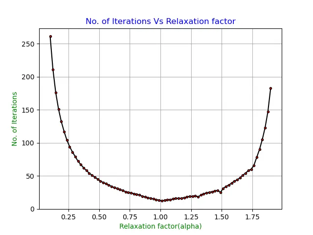
From the graph of No. of Iterations versus Relaxation factor, we can conclude that the curve is rapidly decreasing as we decrease the no. of iterations and the relaxation factor increase and at some point curve become constant at around α=1.0">α=1.0α=1.0 approx. and again the relaxation factor increases with an increase in no. of iteration`
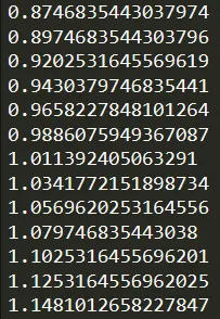
So the value of α">αα lies in the periphery of 1.2 and could be somewhere in between -
Error Encounter:
I do encounter indentation error while writing the program and is shown below.
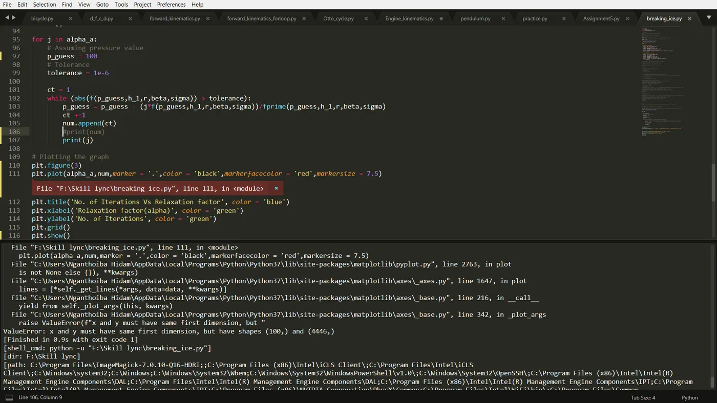
The reason for this error is due to the num values which are iterated inside the while loop has stored inside that same loop without coming out of it. This error could be avoided by removing the spaces before line 105,106,107 so that they are out of while loop and hence values are stored in that and shows the same dimension between alpha_a and num.
Conclusion:
For calculating solutions of non-linear functions and also with comparatively fewer iterations, Newton Raphson Methods shows to be a powerful technique and faster technique too.