Circuit Simulation in VLSI Design: SPICE, Analyses and a Wire-Delay Example
Circuit simulation predicts a chip's voltages and currents before fabrication. How SPICE works, the four core analyses, how SPICE differs from RTL simulation and STA, corners and Monte Carlo, and a 1 mm wire-delay example: 193 ps simulated vs 213 ps lumped vs 189 ps Elmore.
In short
- Circuit simulation predicts how a chip's circuits will behave, with voltages and currents over time, before anything is fabricated. A mistake found after fabrication costs a new set of masks.
- SPICE-type simulators solve the circuit's equations at transistor level, using foundry device models. They run four core analyses: DC operating point, DC sweep, AC small-signal and transient.
- In Skill-Lync's worked example, a 1 mm on-chip wire driven through 1 kΩ reaches 50% of its final voltage after 193 ps in a transient simulation. A one-resistor, one-capacitor model says 213 ps (+10.6%), and the Elmore estimate says 189 ps (−2.4%).
- With 5% random variation in each R and C, 2,000 Monte Carlo runs give a mean delay of 193 ps and a mean + 3σ of 228 ps. Designers sign off against that tail, not the average.
Circuit simulation in VLSI design means calculating, with a computer, how a circuit's voltages and currents will behave before the chip is built. Engineers describe the circuit as a netlist of transistors, resistors and capacitors. They load the foundry's transistor models and ask a simulator such as SPICE for the operating point, frequency response or waveforms over time. They then repeat the run across process, voltage and temperature corners and random variation to check that the design works on every chip, not just a typical one.
This guide explains how a SPICE simulator works, which analyses it runs and where it fits next to faster checks such as RTL simulation and static timing analysis. A worked example then follows a signal down an on-chip wire, so you can see why the model you choose, the time step and process variation all change the answer. Skill-Lync ran every number and figure below in a short Python simulation, and the script is kept with this post.
What is circuit simulation in VLSI design?
Circuit simulation is the numerical solution of a circuit's equations to predict its electrical behaviour before fabrication. In VLSI, transistor-level simulators such as SPICE are used for analog blocks, standard cells, memories and critical paths. Faster gate-level and RTL simulators check the logic of the full chip. Together they catch functional bugs, timing and power problems and sensitivity to variation while fixes are still cheap.
The reason is cost. A chip cannot be patched after the masks are made, and a respin costs a new mask set and months of schedule. So every block is simulated many times: in the typical case, at the extreme corners, and with random device variation. This is the analysis step of the VLSI design flow, repeated at almost every stage.
How does a SPICE simulator work?
SPICE (Simulation Program with Integrated Circuit Emphasis) came out of the University of California, Berkeley. Laurence Nagel's 1975 thesis documents SPICE1 and SPICE2 and the numerical methods behind them, and most circuit simulators used today descend from that work. The open-source ngspice, for example, is based on Berkeley's SPICE3f5. Whatever the tool, a run has the same parts:
- Netlist. A text list of every device and the nodes it connects to, written by hand or exported from a schematic or an extracted layout.
- Device models. Equations that describe how each transistor's current depends on its voltages. Foundries supply them in their process design kit (PDK). For MOSFETs these are usually BSIM models from Berkeley, which an industry body, the Compact Model Coalition, promotes as the standard compact model.
- Equation building. The simulator applies Kirchhoff's current law at every node to get one large system of equations, typically using modified nodal analysis.
- Nonlinear solution. Transistors are nonlinear, so the simulator solves the system iteratively with Newton-Raphson until the node voltages stop changing.
- Time stepping. For a transient run it advances time in small steps, integrating the capacitor and inductor equations numerically and shrinking the step where signals change quickly.
- Output. Waveforms and measured values, such as delays, rise times and power, go to a waveform viewer and to reports.
Which analyses does a circuit simulator run?
Four analyses cover most work. They are the same ones you meet in an analog electronics course, and the ngspice tutorial uses all four.
| Analysis | SPICE command | What it answers | Typical VLSI use |
|---|---|---|---|
| DC operating point | .op | Steady-state node voltages and currents with no signal applied | Bias points of an amplifier or reference; leakage current |
| DC sweep | .dc | How outputs change as a source is stepped | Inverter transfer curve, switching threshold, noise margins |
| AC small-signal | .ac | Gain and phase against frequency, around the operating point | Op-amp bandwidth and phase margin, filter response |
| Transient | .tran | Voltages and currents against time for any input | Gate and wire delay, rise and fall times, power, ring oscillators |
On top of these come noise analysis, corner runs and Monte Carlo runs, described below. If the AC and transient ideas are new, the same RC behaviour appears in this solved GATE question on an RC low-pass filter driven by a square wave.
Is SPICE used to simulate the whole chip?
No. A modern chip has billions of transistors, far too many for transistor-level simulation of every one. Designers use a ladder of methods and trade accuracy for speed at each step:
| Level | What is simulated | Used for |
|---|---|---|
| SPICE (transistor level) | Every transistor with full device models | Analog and RF blocks, standard cells, I/O, critical paths, cell characterisation |
| FastSPICE | Transistors, with simplified models and partitioning | Large memories and mixed-signal blocks too big for SPICE |
| Gate-level simulation | Logic gates with delays from the cell library | Checking the synthesised netlist, including timing annotations |
| RTL simulation | Verilog/VHDL behaviour, cycle by cycle | Functional verification of the whole design |
| Static timing analysis | No simulation: delays of every path are added up | Timing signoff on billions of paths at every corner |
The levels feed each other. SPICE runs characterise each standard cell, meaning they measure its delay and power for many input slopes and loads, and the results go into the cell library. STA and gate-level simulation then use those tables instead of solving transistor equations again. The underlying logic, from CMOS gates up to state machines, is covered in our free Digital Electronics book.
Worked example: how long does a signal take to cross a 1 mm wire?
On-chip wires are not ideal conductors. Each one has resistance along its length and capacitance to its neighbours and to the substrate. On a long wire that adds real delay. Here is the delay of one wire, worked three ways.
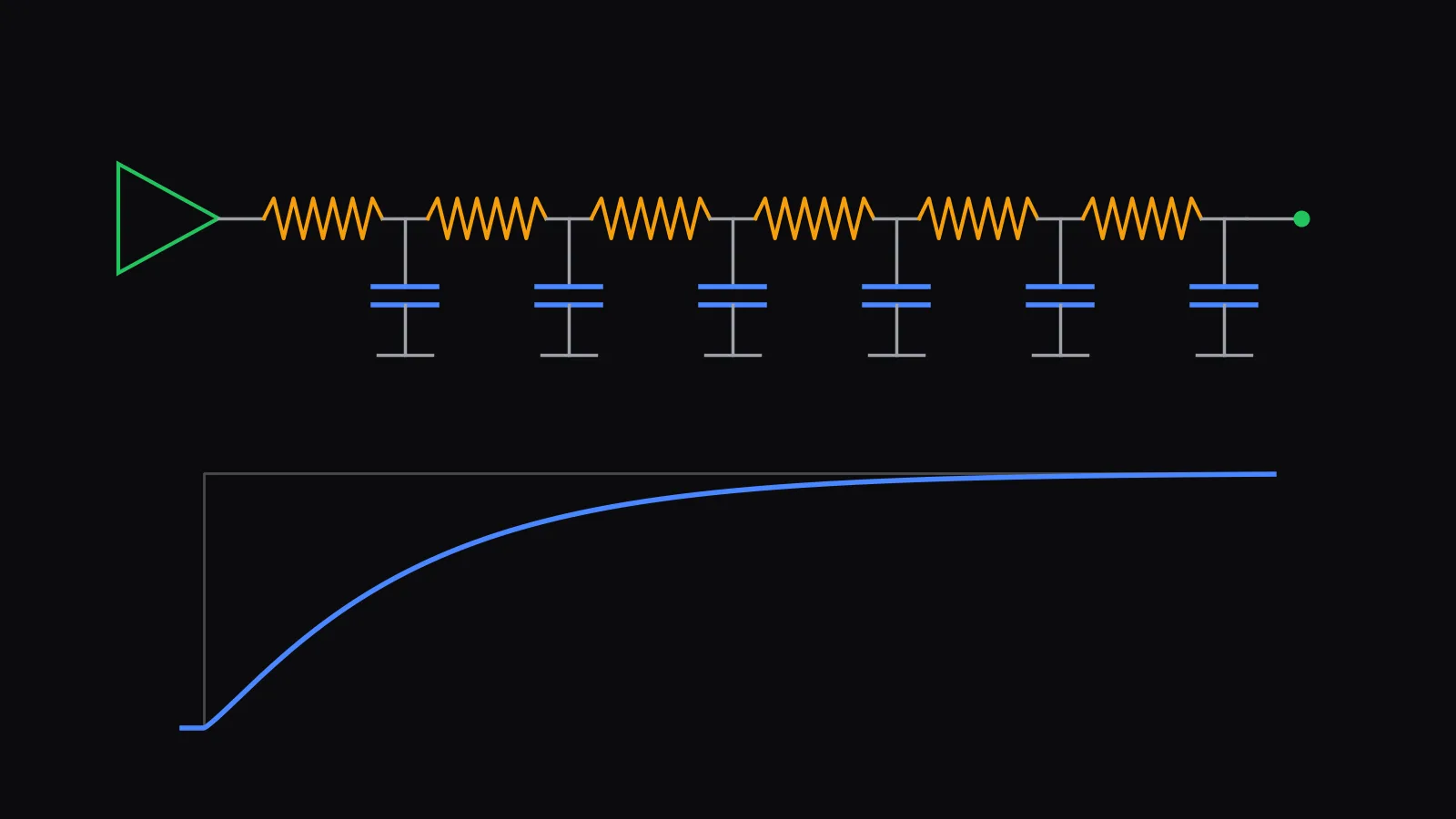
The circuit. A driver with 1 kΩ output resistance switches from 0 to 1 V into a 1 mm wire. The wire has a total resistance and total capacitance fF. At the far end, a gate input adds fF. These are illustrative values chosen to be in a realistic range, not data from a specific foundry process. To simulate the wire, we split it into equal R-C sections, each a small resistor followed by a capacitor to ground.
Estimate 1: the Elmore delay. For an RC ladder, the Elmore delay at a node is the sum, over every capacitor, of that capacitance times the resistance it shares with the path from the source. For our ladder with sections:
The first term is the driver charging all the capacitance. The second is the wire charging itself. The third is the wire resistance charging the load. For a single RC stage, the 50% delay is times RC. Applying the same factor to the Elmore delay gives ps.
Estimate 2: one lumped RC. If the whole wire is treated as one resistor and one capacitor, the RC product is ps, and the 50% delay is ps.
The simulation. A transient simulation of the 10-section ladder, the way SPICE would run it, gives a 50% delay of 193.1 ps.
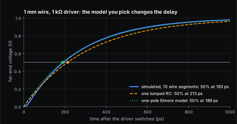
| Model | 50% delay | Error vs 10-section simulation |
|---|---|---|
| Transient simulation, 10 sections | 193.1 ps | reference |
| Transient simulation, 50 sections | 191.0 ps | −1.1% |
| One lumped RC | 213.5 ps | +10.6% |
| 0.69 × Elmore (10 sections) | 188.5 ps | −2.4% |
Two lessons follow. First, how finely you model the wire matters. Lumping it overstates the delay because the far-end load is treated as if it sat behind the whole wire's resistance. Splitting it into more sections converges toward the true distributed answer, which is why extraction tools break long wires into many RC segments. Second, quick formulas such as Elmore are good for estimates and for guiding placement and routing, but signoff numbers come from simulation, or from library tables that simulation produced.
Why does the time step change a transient result?
A transient simulator cannot solve continuously. It advances in time steps and approximates the derivatives at each step. To show the effect, Skill-Lync re-ran the 10-section wire with the simplest method, backward Euler, at fixed steps. A 50 ps step gives a 50% delay of 212.1 ps (+9.8%), a 10 ps step gives 196.9 ps (+2.0%) and a 1 ps step gives 193.5 ps (+0.2%). Production simulators use higher-order integration and adjust the step automatically. Where a signal changes fast they shrink it, and where little happens they grow it. The accuracy settings you choose still decide whether the result can be trusted. A transient run that "passes" with loose tolerances is not proof.
What are corners and Monte Carlo simulation?
No two chips come out of a fab the same. Transistors can be faster or slower, the supply voltage sags, and temperature changes with the surroundings and the chip's own heat. Corner analysis re-runs the simulation at the extremes of process, voltage and temperature (PVT), such as slow transistors at low voltage and high temperature for the worst delay, and fast transistors for the worst hold time and leakage. Monte Carlo analysis adds random, per-device variation. It runs the same circuit hundreds or thousands of times, each time drawing every parameter from its statistical distribution.
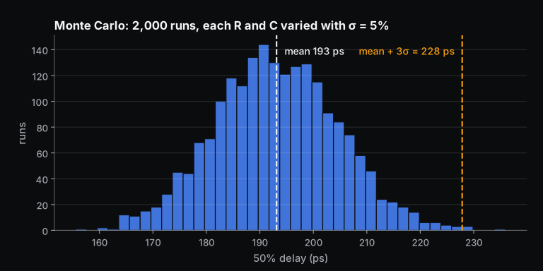
For our wire, giving each of the four R and C values an independent 5% standard deviation and running 2,000 simulations gives a mean delay of 193.1 ps, a standard deviation of 11.6 ps and a range of 155.6 to 235.9 ps. Mean + 3σ is 227.8 ps, 18% above the nominal value. A timing budget built on the 193 ps nominal would fail on a noticeable share of chips. Real foundry Monte Carlo models are correlated and more detailed than this independent 5%, but the lesson is the same: designers sign off against the tail.
Which circuit simulation tools are used in VLSI?
For transistor-level work, the industry's main simulators are Synopsys PrimeSim HSPICE, which Synopsys positions as its signoff accuracy reference, and the Cadence Spectre platform, which spans SPICE, RF, FastSPICE and mixed-signal simulation. For learning and research, free simulators are capable. ngspice is based on Berkeley SPICE3f5. Xyce, from Sandia National Laboratories, is a parallel SPICE-style simulator that supports industry models such as BSIM and PSP. Logic-level simulation uses Verilog and VHDL simulators. The free Icarus Verilog and Verilator are enough to learn RTL simulation, and the companion guide on VLSI design techniques covers the low-power and high-speed methods those simulations verify.
How do you learn circuit simulation for a VLSI career?
Learn the circuits before the tool. RC charging, the MOSFET as a switch and an amplifier, and CMOS inverter behaviour are what a simulator's output is checked against. If a waveform surprises you, you need to know whether the circuit or the setup is wrong. Practise with ngspice on small circuits first: an RC filter (.ac and .tran), an inverter transfer curve (.dc), then a ring oscillator. The solved GATE question on MOSFET switch logic and power is a good warm-up for the digital side.
Skill-Lync's Basics of Digital Electronics course is an 11-week online course with 22 hours of content and 2 projects. It runs from number systems and CMOS logic through combinational and sequential circuits, state machines and programmable logic, and it includes simulation-based design verification. For where these skills lead, see our guide to India's semiconductor mission and VLSI jobs, or talk to a Skill-Lync counsellor about which track fits you.
Frequently asked questions
What is SPICE simulation in VLSI?
SPICE simulation solves a circuit's equations at transistor level, using the foundry's device models, to predict voltages and currents. In VLSI it is used for analog blocks, standard cells, memories, I/O and critical timing paths. Its main analyses are DC operating point, DC sweep, AC small-signal and transient, plus corner and Monte Carlo runs for variation.
What is the difference between circuit simulation and static timing analysis?
Circuit simulation computes actual waveforms for given inputs, which is accurate but slow, and it only covers the cases you simulate. Static timing analysis does not simulate. It adds up pre-characterised cell and wire delays along every path and checks them against the clock, so it covers billions of paths quickly. STA's delay tables come from SPICE characterisation of each cell.
What is transient analysis?
Transient analysis computes how voltages and currents change over time after an input changes, such as a clock edge or a step. The simulator advances in small time steps and integrates the circuit equations numerically. It is the analysis used to measure gate and wire delays, rise and fall times, glitches and dynamic power.
Why is Monte Carlo simulation used in chip design?
Manufacturing makes every transistor and wire slightly different. Monte Carlo simulation runs the same circuit many times with parameters drawn from their statistical distributions, to show the spread of delay, offset or power. Designers then check that the worst likely case, often around mean plus 3σ, still meets the specification, so that the yield is acceptable.
Is ngspice good enough to learn circuit simulation?
Yes. ngspice is free, is based on Berkeley SPICE3f5 and supports the standard DC, AC and transient analyses, so the skills transfer directly to commercial simulators. What you will not get with it is a commercial foundry's PDK. Open PDKs and textbook models are enough to learn analysis, convergence and measurement.
What is the Elmore delay?
The Elmore delay is a quick estimate of the delay through an RC network. For each capacitor, multiply it by the resistance it shares with the path from the driver, then add the results. Multiplying by 0.69 gives an approximate 50% delay. In our 1 mm wire example, that gives 188.5 ps, against 193.1 ps from simulation.
Sources and further reading
- L. W. Nagel, SPICE2: A Computer Program to Simulate Semiconductor Circuits, UC Berkeley ERL M520, 1975
- ngspice, documentation and tutorial (op, dc, ac and tran analyses)
- BSIM Group, UC Berkeley, BSIM compact models
- Wikipedia, Elmore delay (W. C. Elmore, 1948)
- Wikipedia, Static timing analysis (corners)
- Synopsys, PrimeSim HSPICE; Cadence, Spectre Simulation Platform; Sandia, Xyce paper
- Skill-Lync, VLSI design flow: 13 steps from specification to tapeout